Describing data with graphics and numbers Types of

Describing data with graphics and numbers

Types of Data • Categorical Variables – also known as class variables, nominal variables • Quantitative Variables – aka numerical nariables – either continuous or discrete.

Graphing categorical variables

Ten most common causes of death in Americans between 15 and 19 years old in 1999.

Bar graphs

Graphing numerical variables

Heights of BIOL 300 students (cm) 165 170 142 173 168 155 160 165 163 152 154 165 180 173 190 165 175 165 170 156 155 163 168 177 166

Stem-and-leaf plot

Stem-and-leaf plot 19 18 17 16 15 14 0 0 0003357 0335555556888 24556 2

Frequency table Height Group 141 -150 151 -160 161 -170 171 -180 181 -190 Frequency

Frequency table Height Group Frequency 141 -150 1 151 -160 6 161 -170 15 171 -180 5 181 -190 1

Histogram

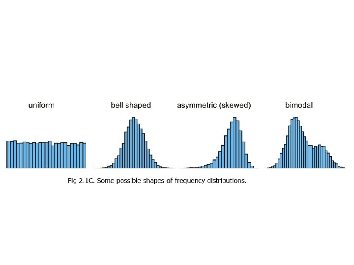
Histogram Frequency distribution

Histogram with more data

50 th percentile (median) 90 th percentile

Associations between two categorical variables

Association between reproductive effort and avian malaria

Mosaic plot

Grouped Bar Graph

Associations between categorical and numerical variables

Multiple histograms

Associations between two numerical variables

Scatterplots

Evaluating Graphics • Lie factor • Chartjunk • Efficiency

Don’t mislead with graphics

Better representation of truth

Lie Factor • Lie factor = size of effect shown in graphic size of effect in data

Lie Factor Example Effect in graphic: 2. 33/0. 08 = 29. 1 Effect in data: 6748/5844 = 1. 15 Lie factor = 29. 1 / 1. 15 = 25. 3

Chartjunk

Needless 3 D Graphics

Summary: Graphical methods for frequency distributions

Summary: Associations between variables

Great book on graphics

Describing data

Two common descriptions of data • Location (or central tendency) • Width (or spread)

Measures of location Mean Median Mode

Mean n is the size of the sample

Mean Y 1=56, Y 2=72, Y 3=18, Y 4=42

Mean Y 1=56, Y 2=72, Y 3=18, Y 4=42 = (56+72+18+42) / 4 = 47

Median • The median is the middle measurement in a set of ordered data.

The data: 18 28 24 25 36 14 34

The data: 18 28 24 25 36 14 34 can be put in order: 14 18 24 Median is 25. 25 28 34 36

Mean vs. median in politics • 2004 U. S. Economy • Republicans: times are good – Mean income increasing ~ 4% per year • Democrats: times are bad – Median family income fell • Why?

Measures of width • • Range Standard deviation Variance Coefficient of variation

Range 14 17 18 20 22 22 24 25 26 28 28 28 30 34 36

Range 14 17 18 20 22 22 24 25 26 28 28 28 30 34 36 The range is 36 -14 = 22

Population Variance

Sample variance n is the sample size

Shortcut for calculating sample variance

Standard deviation (SD) • Positive square root of the variance s is the true standard deviation s is the sample standard deviation

In class exercise Calculate the variance and standard deviation of a sample with the following data: 6, 1, 2

Answer Variance=7 Standard deviation =

Coefficient of variance (CV) CV = 100 s / .

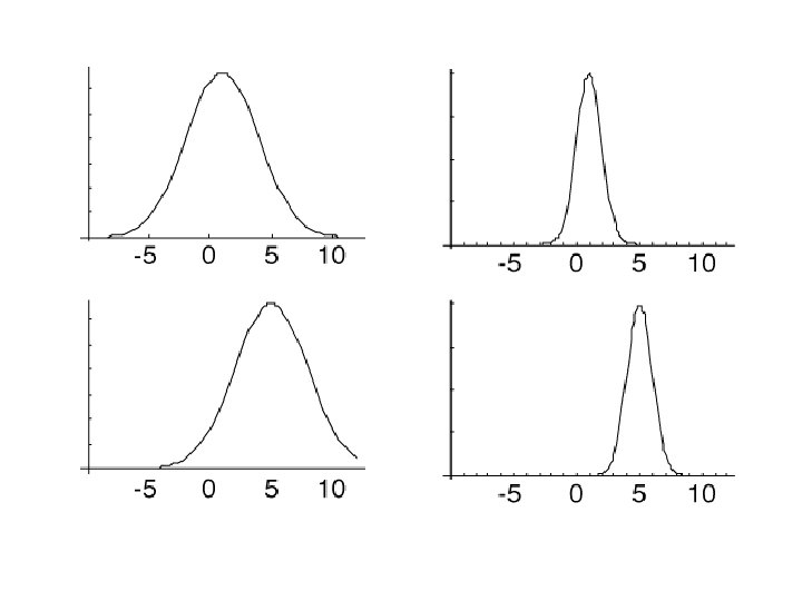
Equal means, different variances

Manipulating means • The mean of the sum of two variables: E[X + Y] = E[X]+ E[Y] • The mean of the sum of a variable and a constant: E[X + c] = E[X]+ c • The mean of a product of a variable and a constant: E[c X] = c E[X] • The mean of a product of two variables: E[X Y] = E[X] E[Y] if and only if X and Y are independent.

Manipulating variance • The variance of the sum of two variables: Var[X + Y] = Var[X]+ Var[Y] if and only if X and Y are independent. • The variance of the sum of a variable and a constant: Var[X + c] = Var[X] • The variance of a product of a variable and a constant: Var[c X] = c 2 Var[X]

Parents’ heights Mean Variance Father Height 174. 3 71. 7 Mother Height 160. 4 58. 3 Father Height +Mother Height 334. 7 184. 9