Describing Data Using Numerical Measures 3 1 Learning

Describing Data Using Numerical Measures 3 -1

Learning Outcomes Outcome 1. Compute the mean, median, mode, and weighted mean for a set of data and understand what these values represent. Outcome 2. Construct a box and whisker graph and interpret it. Outcome 3. Compute the range, interquartile range, variance, and standard deviation and know what these values mean. Outcome 4. Compute a z score and the coefficient of variation and understand how they are applied in decision-making situations. Outcome 5. Understand the Empirical Rule and Tchebysheff’s Theorem. 3 -2

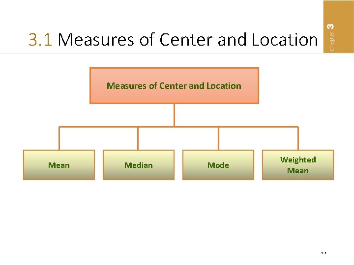
3. 1 Measures of Center and Location Mean Median Mode Weighted Mean 3 -3

Parameter and Statistic • Parameter – A measure computed from the entire population – As long as the population does not change, the value of the parameter will not change • Statistic – A measure computed from a sample that has been selected from a population – The value of the statistic will depend on which sample is selected. 3 -4

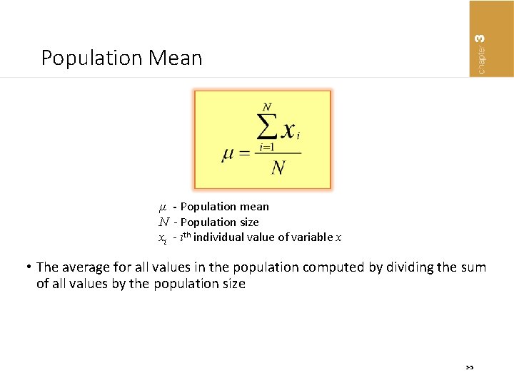
Population Mean µ - Population mean N - Population size xi - ith individual value of variable x • The average for all values in the population computed by dividing the sum of all values by the population size 3 -5

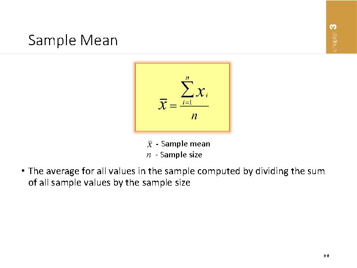
Sample Mean - Sample mean n - Sample size • The average for all values in the sample computed by dividing the sum of all sample values by the sample size 3 -6

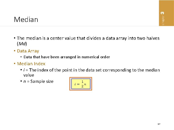
Median • The median is a center value that divides a data array into two halves (Md) • Data Array • Data that have been arranged in numerical order • Median Index • i = The index of the point in the data set corresponding to the median value • n = Sample size 3 -7

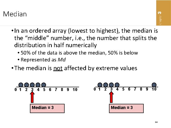
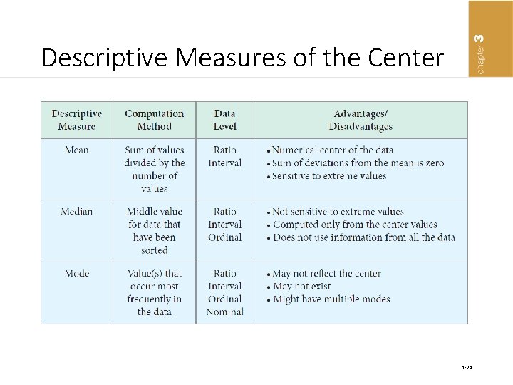
Median • In an ordered array (lowest to highest), the median is the “middle” number, i. e. , the number that splits the distribution in half numerically • 50% of the data is above the median, 50% is below • Represented as Md • The median is not affected by extreme values 0 1 2 3 4 5 6 7 8 9 10 0 1 2 3 4 5 6 7 Median = 3 8 9 10 Median = 3 3 -8

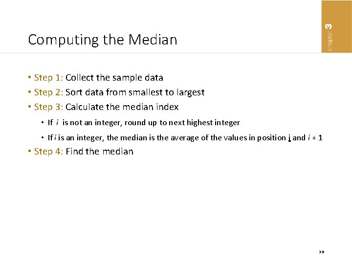
Computing the Median • Step 1: Collect the sample data • Step 2: Sort data from smallest to largest • Step 3: Calculate the median index • If i is not an integer, round up to next highest integer • If i is an integer, the median is the average of the values in position i and i + 1 • Step 4: Find the median 3 -9

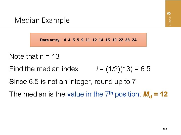
Median Example Data array: 4 4 5 5 9 11 12 14 16 19 22 23 24 Note that n = 13 Find the median index i = (1/2)(13) = 6. 5 Since 6. 5 is not an integer, round up to 7 The median is the value in the 7 th position: Md = 12 3 -10

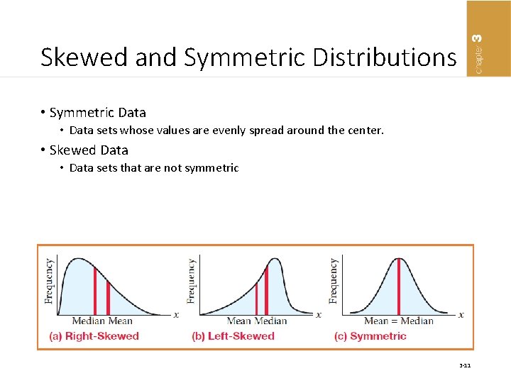
Skewed and Symmetric Distributions • Symmetric Data • Data sets whose values are evenly spread around the center. • Skewed Data • Data sets that are not symmetric 3 -11

Mode • The value in a data set that occurs most frequently • Is not affected by extreme values • Can be used for both quantitative and qualitative data • Can have more than one mode, or no mode • Distribution with two modes - bimodal 3 -12

The “Best” Measure • Mean is generally used, unless extreme values (outliers) exist • Then Median is often used, since the median is not sensitive to extreme values. • Example: Median home prices may be reported for a region – less sensitive to outliers • Mode is good for determining more likely to occur 3 -13

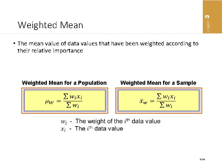
Weighted Mean • The mean value of data values that have been weighted according to their relative importance Weighted Mean for a Population Weighted Mean for a Sample 3 -14

Calculating Weighted Mean • Step 1: Collect the desired data and determine the weight to be assigned to each data value • Step 2: Multiply each weight by the data value and sum these • Step 3: Sum weights for all values • Step 4: Compute the weighted mean 3 -15

Percentiles and Quartiles Percentiles The pth percentile in a data array: • p% are less than or equal to this value • (100 – p)% are greater than or equal to this value (where 0 ≤ p ≤ 100) Quartiles 1 st quartile = 25 th percentile 2 nd quartile = 50 th percentile Also the median 3 rd quartile = 75 th percentile • 50 th percentile is the median 3 -16

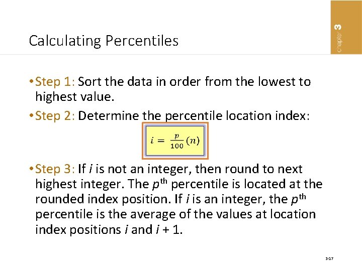
Calculating Percentiles • Step 1: Sort the data in order from the lowest to highest value. • Step 2: Determine the percentile location index: • Step 3: If i is not an integer, then round to next highest integer. The pth percentile is located at the rounded index position. If i is an integer, the pth percentile is the average of the values at location index positions i and i + 1. 3 -17

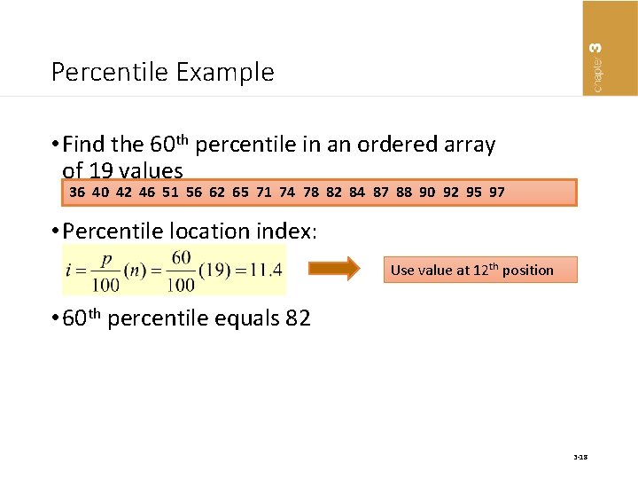
Percentile Example • Find the 60 th percentile in an ordered array of 19 values 36 40 42 46 51 56 62 65 71 74 78 82 84 87 88 90 92 95 97 • Percentile location index: Use value at 12 th position • 60 th percentile equals 82 3 -18

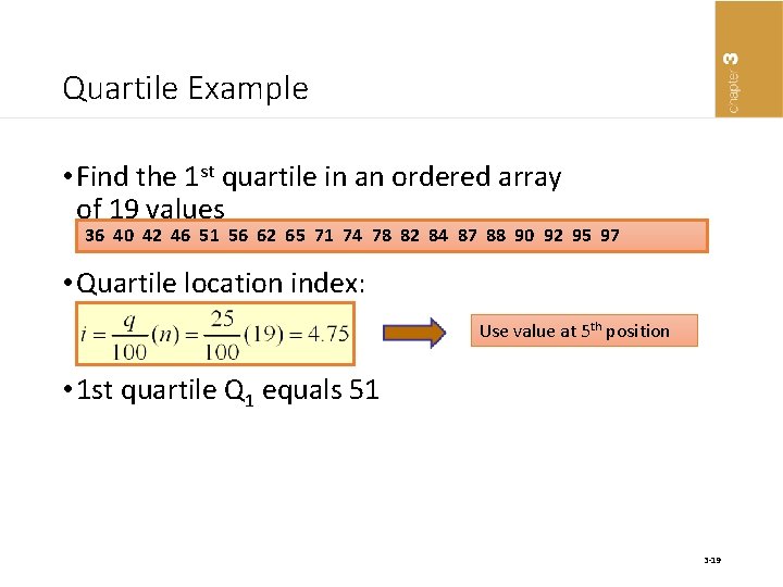
Quartile Example • Find the 1 st quartile in an ordered array of 19 values 36 40 42 46 51 56 62 65 71 74 78 82 84 87 88 90 92 95 97 • Quartile location index: Use value at 5 th position • 1 st quartile Q 1 equals 51 3 -19

Box and Whisker Plot • A graph that is composed of two parts: a box and the whiskers • The box has a width that ranges from the first quartile (Q 1) to the third quartile (Q 3) • A vertical line through the box is placed at the median. • Limits are located at a value that is 1. 5 multiplied by the difference between Q 1 and Q 3 below Q 1 and above Q 3. • The whiskers extend to the left to the lowest value within the limits and to the right to the highest value within the limits. 3 -20

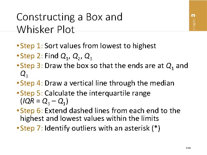
Constructing a Box and Whisker Plot • Step 1: Sort values from lowest to highest • Step 2: Find Q 1, Q 2, Q 3 • Step 3: Draw the box so that the ends are at Q 1 and Q 3 • Step 4: Draw a vertical line through the median • Step 5: Calculate the interquartile range (IQR = Q 3 – Q 1) • Step 6: Extend dashed lines from each end to the highest and lowest values within the limits • Step 7: Identify outliers with an asterisk (*) 3 -21

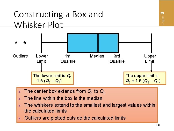
Constructing a Box and Whisker Plot * * Outliers Lower 1 st Median 3 rd Upper Limit Quartile Limit The lower limit is Q 1 – 1. 5 (Q 3 – Q 1) n n The upper limit is Q 3 + 1. 5 (Q 3 – Q 1) The center box extends from Q 1 to Q 3 The line within the box is the median The whiskers extend to the smallest and largest values within the calculated limits Outliers are plotted outside the calculated limits 3 -22

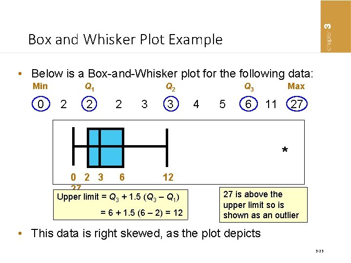
Box and Whisker Plot Example • Below is a Box-and-Whisker plot for the following data: Min Q 1 Q 2 Q 3 Max 0 2 2 2 3 3 4 5 6 11 27 * 0 2 3 27 6 12 Upper limit = Q 3 + 1. 5 (Q 3 – Q 1) = 6 + 1. 5 (6 – 2) = 12 27 is above the upper limit so is shown as an outlier • This data is right skewed, as the plot depicts 3 -23

Descriptive Measures of the Center 3 -24

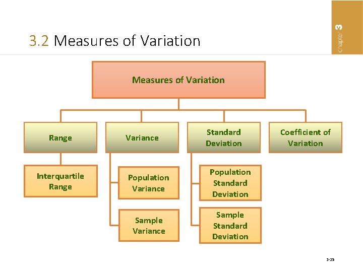
3. 2 Measures of Variation Range Interquartile Range Variance Standard Deviation Population Variance Population Standard Deviation Sample Variance Sample Standard Deviation Coefficient of Variation 3 -25

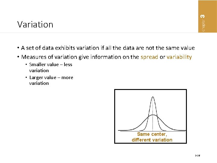
Variation • A set of data exhibits variation if all the data are not the same value • Measures of variation give information on the spread or variability • Smaller value – less variation • Larger value – more variation Same center, different variation 3 -26

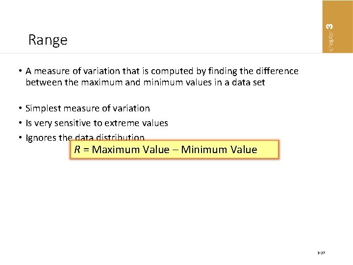
Range • A measure of variation that is computed by finding the difference between the maximum and minimum values in a data set • Simplest measure of variation • Is very sensitive to extreme values • Ignores the data distribution R = Maximum Value – Minimum Value 3 -27

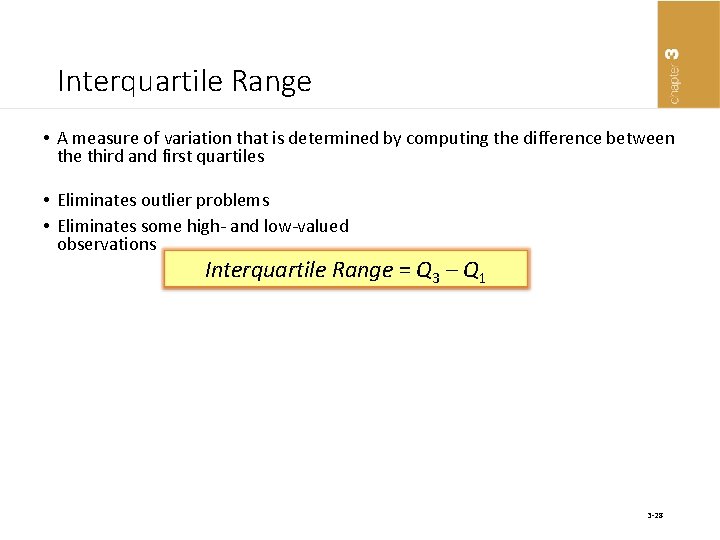
Interquartile Range • A measure of variation that is determined by computing the difference between the third and first quartiles • Eliminates outlier problems • Eliminates some high- and low-valued observations Interquartile Range = Q 3 – Q 1 3 -28

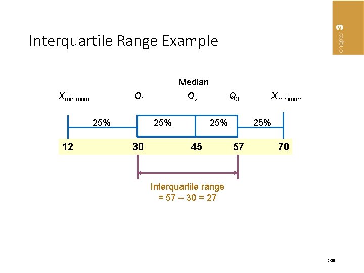
Interquartile Range Example Median Xminimum Q 1 Q 2 Q 3 Xminimum 25% 25% 12 30 45 57 70 Interquartile range = 57 – 30 = 27 3 -29

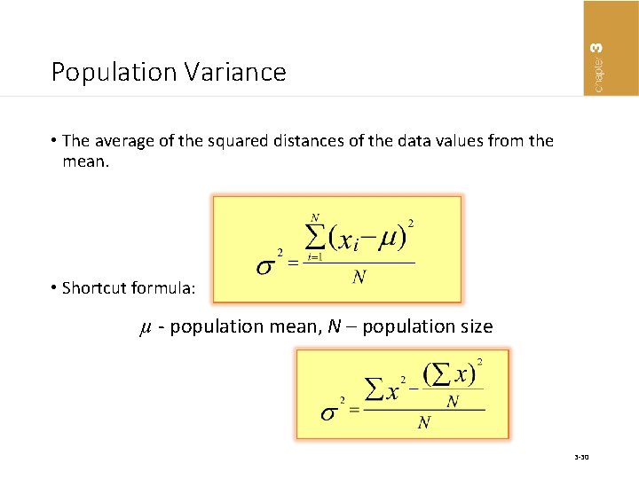
Population Variance • The average of the squared distances of the data values from the mean. • Shortcut formula: µ - population mean, N – population size 3 -30

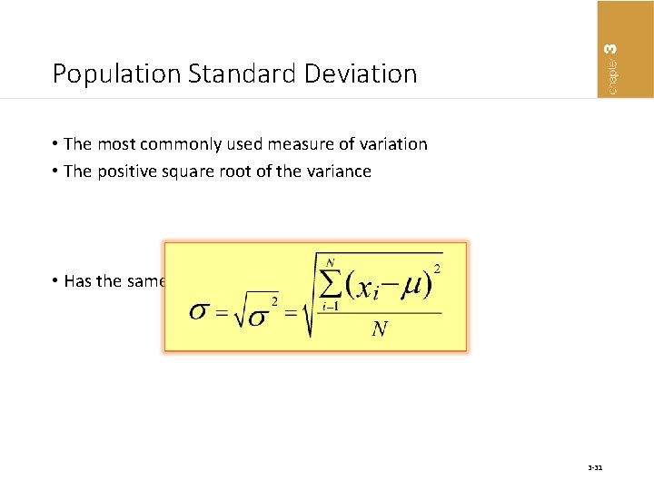
Population Standard Deviation • The most commonly used measure of variation • The positive square root of the variance • Has the same units as the original data 3 -31

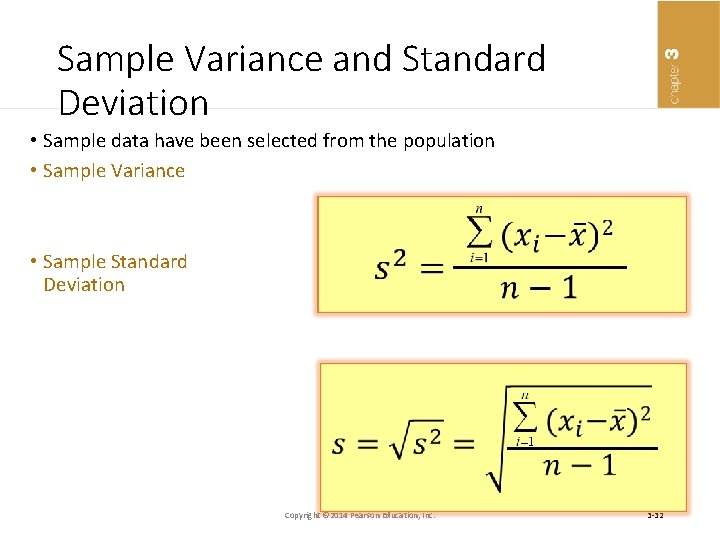
Sample Variance and Standard Deviation • Sample data have been selected from the population

Computing Sample Variance and Standard Deviation • Step 1: Select the sample and record the data for the variable of interest • Step 2: Select expression for sample variance • Step 3: Compute x • Step 4: Determine the sum of the squared deviations of each x value from x • Step 5: Compute the sample variance • Step 6: Compute the sample standard deviation by taking the square root of the variance 3 -33

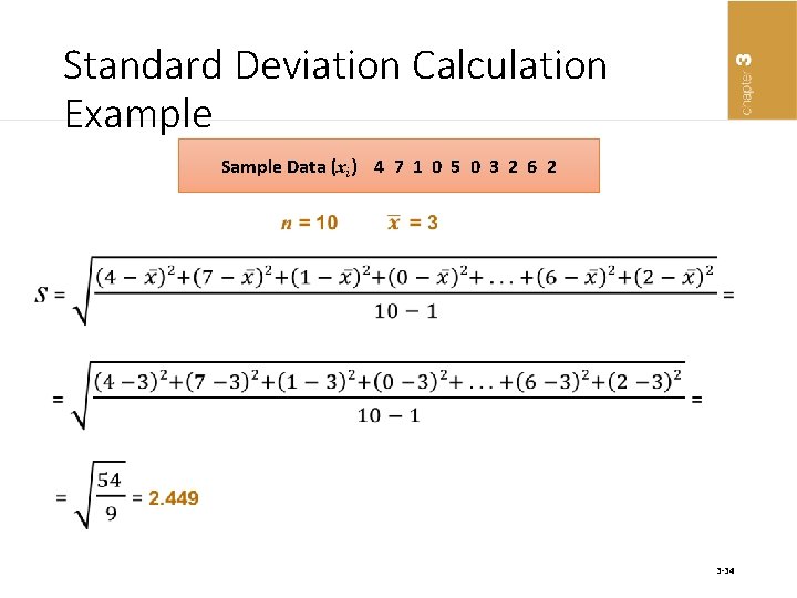
Standard Deviation Calculation Example Sample Data (xi) 4 7 1 0 5 0 3 2 6 2 3 -34

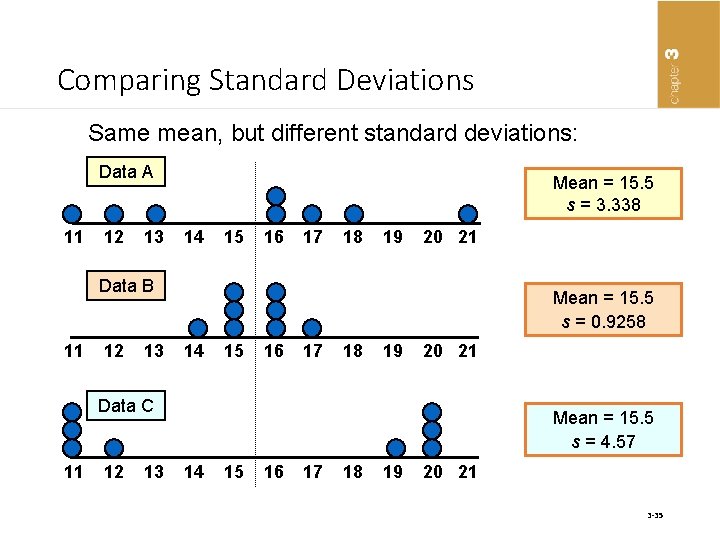
Comparing Standard Deviations Same mean, but different standard deviations: Data A 11 12 13 Mean = 15. 5 s = 3. 338 14 15 16 17 18 19 20 21 Data B 11 12 13 Mean = 15. 5 s = 0. 9258 14 15 16 17 18 19 20 21 Data C 11 12 13 Mean = 15. 5 s = 4. 57 14 15 16 17 18 19 20 21 3 -35

3. 3 Using the Mean and Standard Deviation Together • Coefficient of Variation (CV) • The ratio of the standard deviation to the mean expressed as a percentage. The coefficient of variation is used to measure variation relative to the mean • Measures relative variation • Always expressed in percentage (%) • Shows variation relative to mean 3 -36

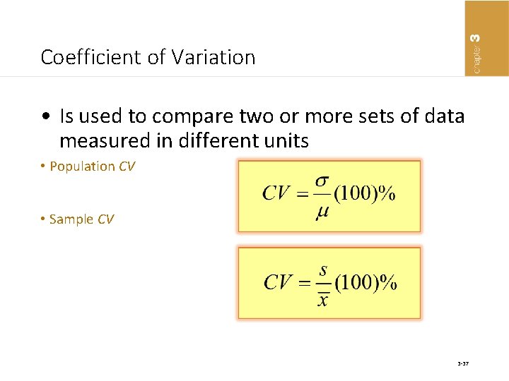
Coefficient of Variation • Is used to compare two or more sets of data measured in different units • Population CV • Sample CV 3 -37

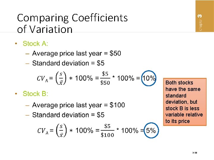
Comparing Coefficients of Variation • Both stocks have the same standard deviation, but stock B is less variable relative to its price 3 -38

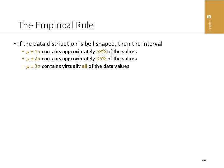
The Empirical Rule • If the data distribution is bell shaped, then the interval • µ ± 1σ contains approximately 68% of the values • µ ± 2σ contains approximately 95% of the values • µ ± 3σ contains virtually all of the data values 3 -39

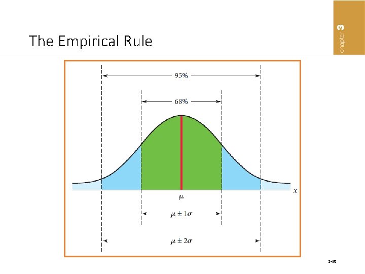
The Empirical Rule 3 -40

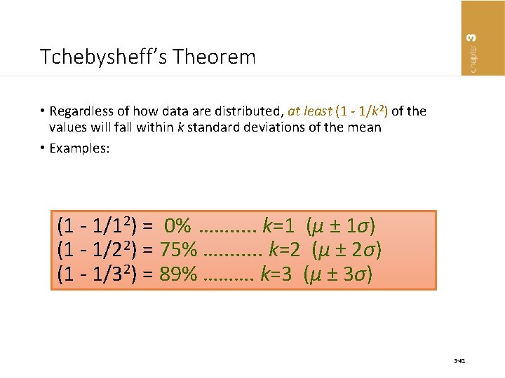
Tchebysheff’s Theorem • Regardless of how data are distributed, at least (1 - 1/k 2) of the values will fall within k standard deviations of the mean • Examples: (1 - 1/12) = 0% ……. . . k=1 (μ ± 1σ) (1 - 1/22) = 75% …. . . . k=2 (μ ± 2σ) (1 - 1/32) = 89% ………. k=3 (μ ± 3σ) 3 -41

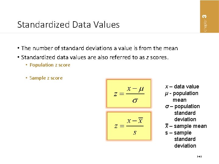
Standardized Data Values • The number of standard deviations a value is from the mean • Standardized data values are also referred to as z scores. • Population z score • Sample z score x – data value µ - population mean σ – population standard deviation x – sample mean s – sample standard deviation 3 -42

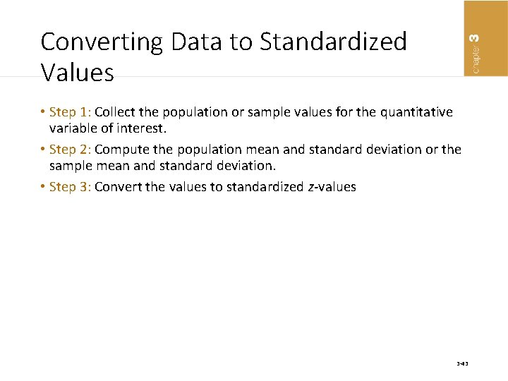
Converting Data to Standardized Values • Step 1: Collect the population or sample values for the quantitative variable of interest. • Step 2: Compute the population mean and standard deviation or the sample mean and standard deviation. • Step 3: Convert the values to standardized z-values 3 -43

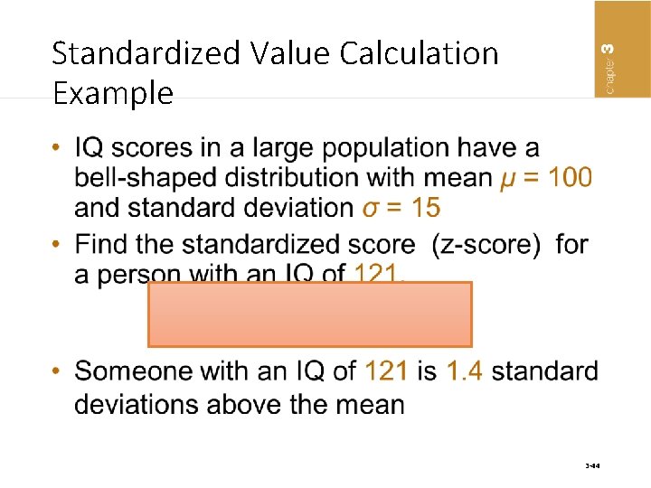
Standardized Value Calculation Example • 3 -44

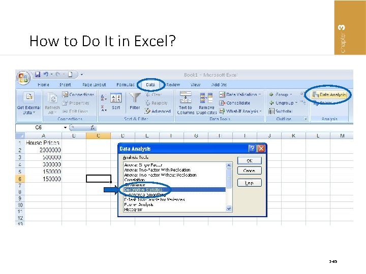
How to Do It in Excel? 3 -45

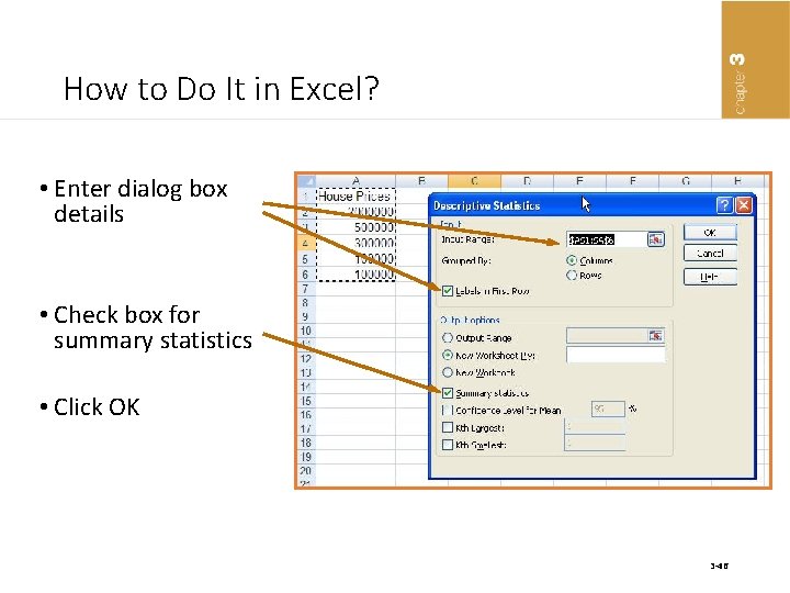
How to Do It in Excel? • Enter dialog box details • Check box for summary statistics • Click OK 3 -46

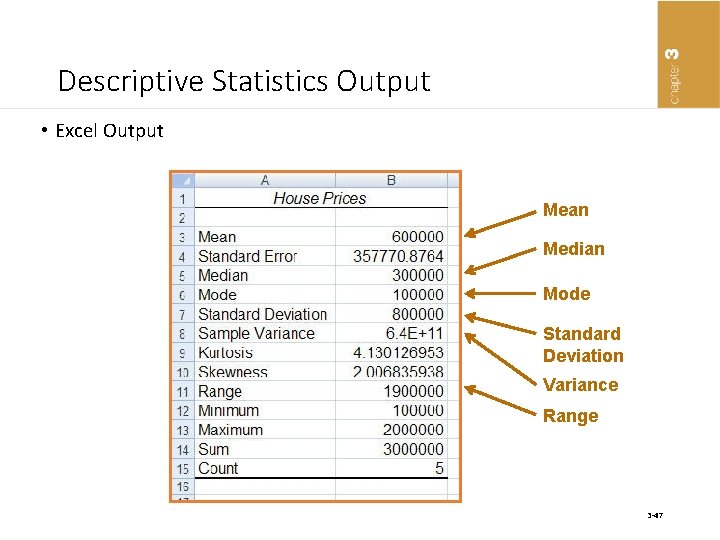
Descriptive Statistics Output • Excel Output Mean Median Mode Standard Deviation Variance Range 3 -47