Dependent Sample t test Independent Samples t test

Dependent Sample t test Independent Samples t test 11/13/14

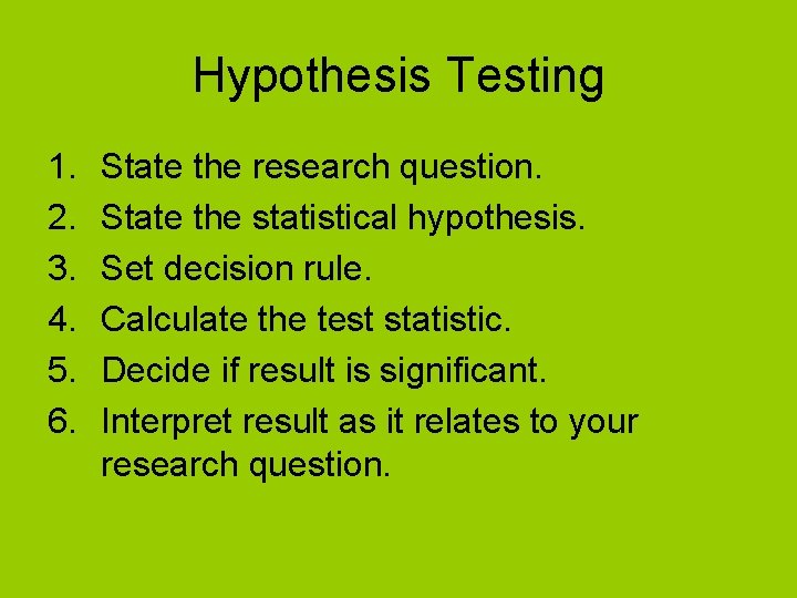
Hypothesis Testing 1. 2. 3. 4. 5. 6. State the research question. State the statistical hypothesis. Set decision rule. Calculate the test statistic. Decide if result is significant. Interpret result as it relates to your research question.

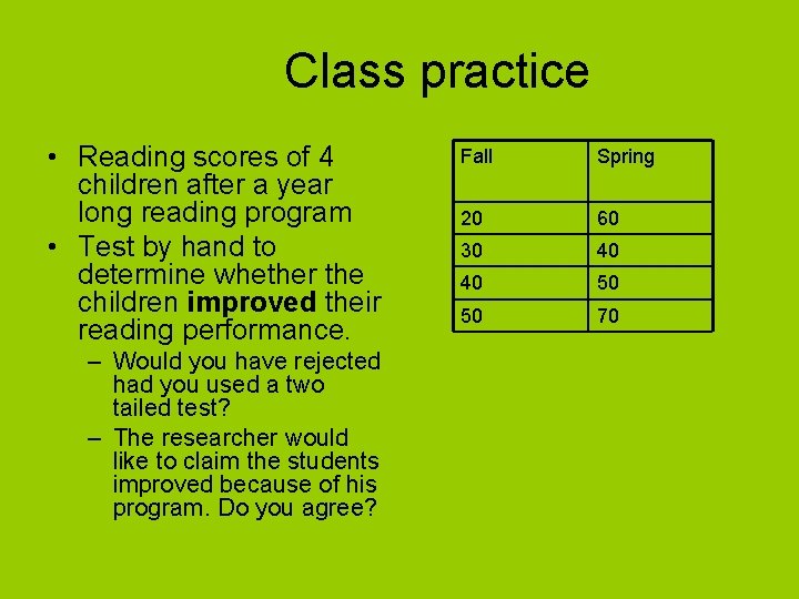
Class practice • Reading scores of 4 children after a year long reading program • Test by hand to determine whether the children improved their reading performance. – Would you have rejected had you used a two tailed test? – The researcher would like to claim the students improved because of his program. Do you agree? Fall Spring 20 60 30 40 40 50 50 70

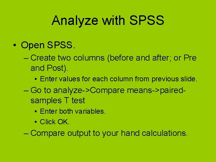
Analyze with SPSS • Open SPSS. – Create two columns (before and after; or Pre and Post). • Enter values for each column from previous slide. – Go to analyze->Compare means->pairedsamples T test • Enter both variables. • Click OK. – Compare output to your hand calculations.

Issues with Repeated Measures Designs • Order effects. – Use counterbalancing in order to eliminate any potential bias in favor of one condition because most subjects happen to experience it first (order effects). – Randomly assign half of the subjects to experience the two conditions in a particular order. • Practice effects. – Do not repeat measurement if effects linger.

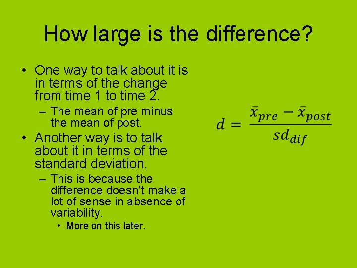
How large is the difference? • One way to talk about it is in terms of the change from time 1 to time 2. – The mean of pre minus the mean of post. • Another way is to talk about it in terms of the standard deviation. – This is because the difference doesn’t make a lot of sense in absence of variability. • More on this later.

Independent Samples T test

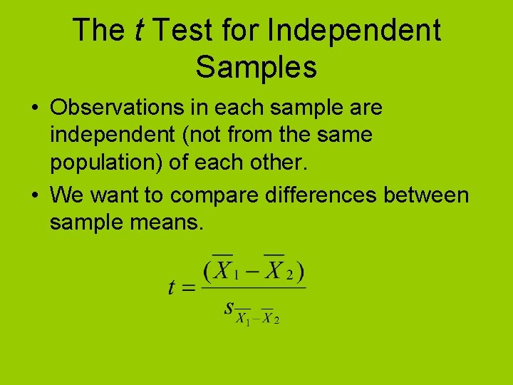
The t Test for Independent Samples • Observations in each sample are independent (not from the same population) of each other. • We want to compare differences between sample means.

Sampling Distribution of the Difference Between Means • Imagine repeatedly gathering two random samples from a population. – Each time subtracting one from the other. • If you create a sampling distribution of the difference between the means… – Given the null hypothesis, we expect the mean of the sampling distribution of differences, 1 - 2, to be 0. – We must estimate the standard deviation of the sampling distribution of the difference between means.

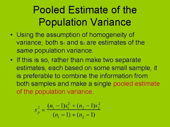
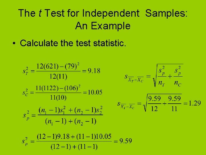
Pooled Estimate of the Population Variance • Using the assumption of homogeneity of variance, both s 1 and s 2 are estimates of the same population variance. • If this is so, rather than make two separate estimates, each based on some small sample, it is preferable to combine the information from both samples and make a single pooled estimate of the population variance.

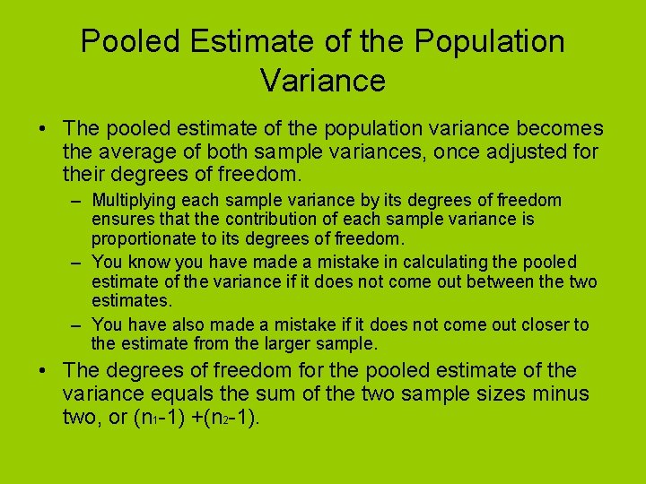
Pooled Estimate of the Population Variance • The pooled estimate of the population variance becomes the average of both sample variances, once adjusted for their degrees of freedom. – Multiplying each sample variance by its degrees of freedom ensures that the contribution of each sample variance is proportionate to its degrees of freedom. – You know you have made a mistake in calculating the pooled estimate of the variance if it does not come out between the two estimates. – You have also made a mistake if it does not come out closer to the estimate from the larger sample. • The degrees of freedom for the pooled estimate of the variance equals the sum of the two sample sizes minus two, or (n 1 -1) +(n 2 -1).

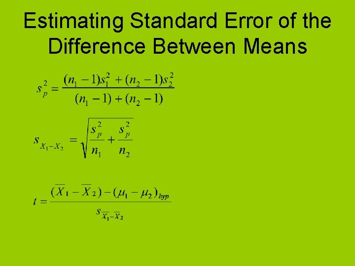
Estimating Standard Error of the Difference Between Means

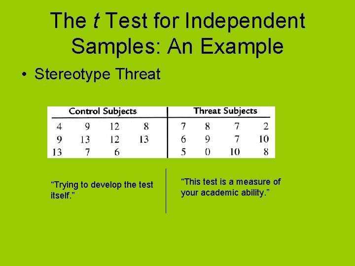
The t Test for Independent Samples: An Example • Stereotype Threat “Trying to develop the test itself. ” “This test is a measure of your academic ability. ”

Hypothesis Testing 1. 2. 3. 4. 5. 6. State the research question. State the statistical hypothesis. Set decision rule. Calculate the test statistic. Decide if result is significant. Interpret result as it relates to your research question.

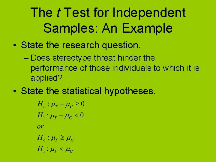
The t Test for Independent Samples: An Example • State the research question. – Does stereotype threat hinder the performance of those individuals to which it is applied? • State the statistical hypotheses.

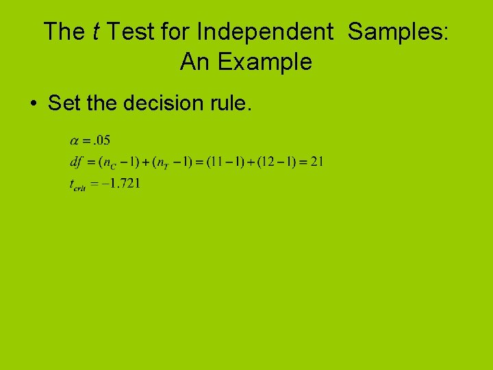
The t Test for Independent Samples: An Example • Set the decision rule.

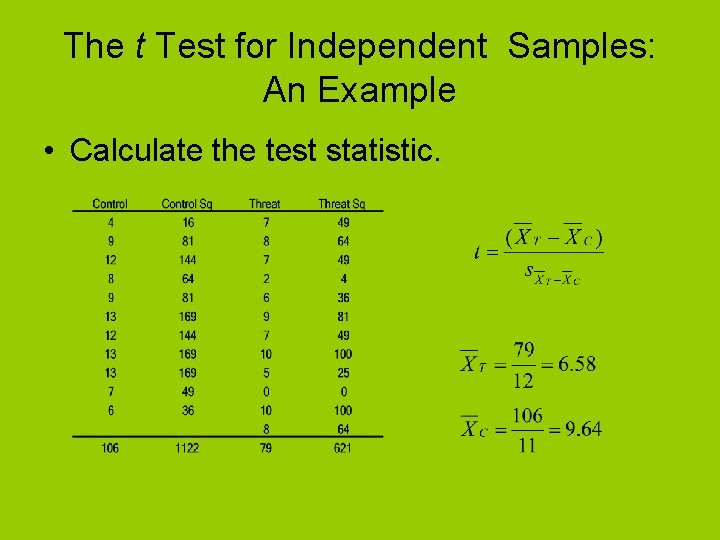
The t Test for Independent Samples: An Example • Calculate the test statistic.

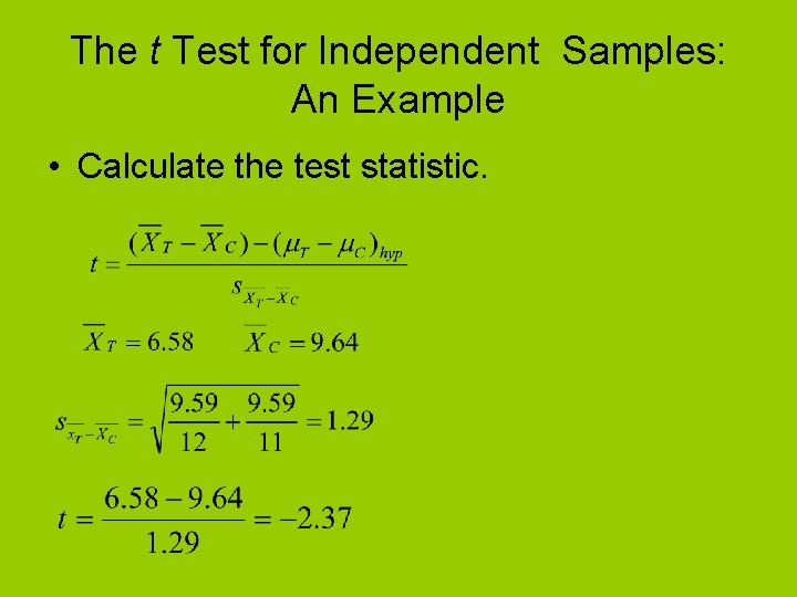
The t Test for Independent Samples: An Example • Calculate the test statistic.

The t Test for Independent Samples: An Example • Calculate the test statistic.

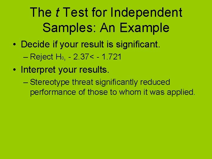
The t Test for Independent Samples: An Example • Decide if your result is significant. – Reject H 0, - 2. 37< - 1. 721 • Interpret your results. – Stereotype threat significantly reduced performance of those to whom it was applied.

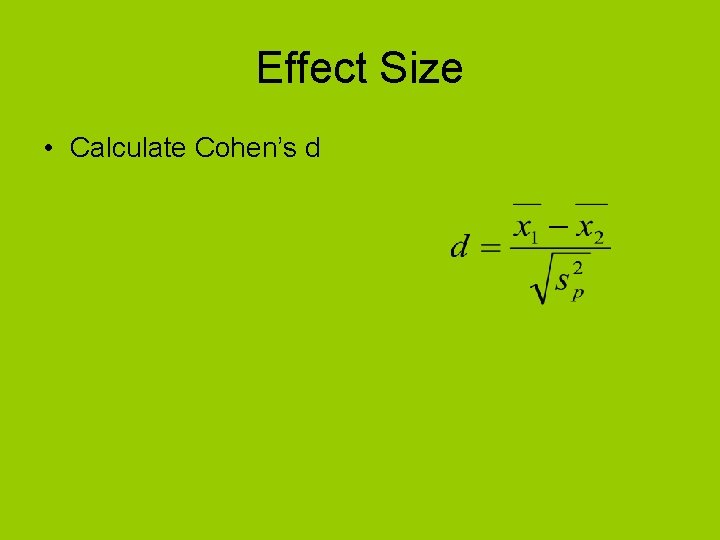
Effect Size • Calculate Cohen’s d

More on Cohen’s d

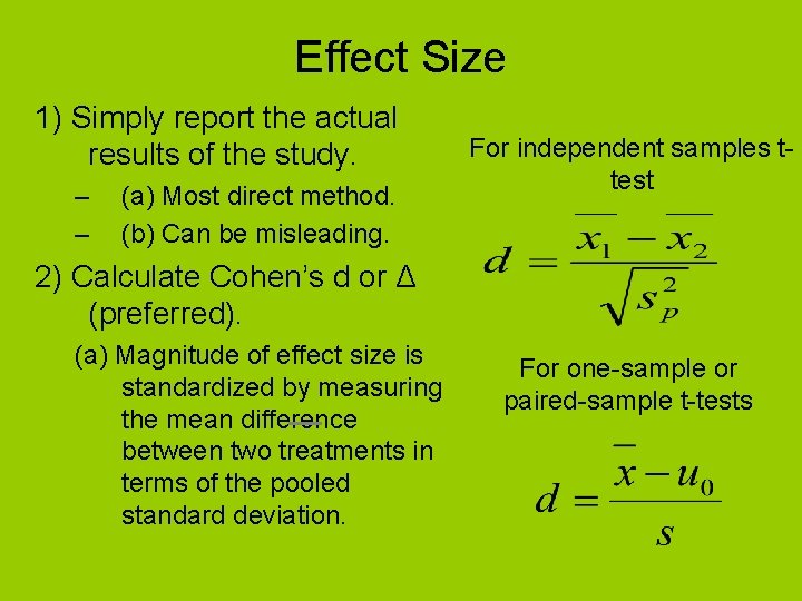
Effect Size 1) Simply report the actual results of the study. – – (a) Most direct method. (b) Can be misleading. For independent samples ttest 2) Calculate Cohen’s d or Δ (preferred). (a) Magnitude of effect size is standardized by measuring the mean difference between two treatments in terms of the pooled standard deviation. For one-sample or paired-sample t-tests

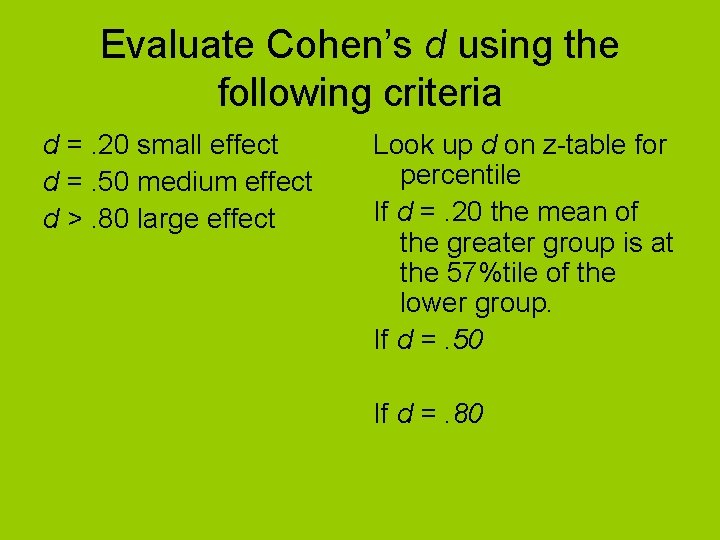
Evaluate Cohen’s d using the following criteria d =. 20 small effect d =. 50 medium effect d >. 80 large effect Look up d on z-table for percentile If d =. 20 the mean of the greater group is at the 57%tile of the lower group. If d =. 50 If d =. 80

Another example See handout

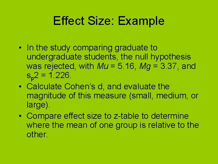
Effect Size: Example • In the study comparing graduate to undergraduate students, the null hypothesis was rejected, with Mu = 5. 16, Mg = 3. 37, and sp 2 = 1. 226. • Calculate Cohen’s d, and evaluate the magnitude of this measure (small, medium, or large). • Compare effect size to z-table to determine where the mean of one group is relative to the other.

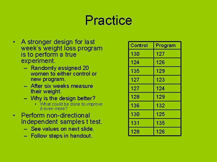
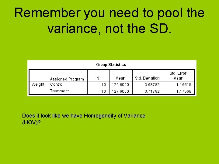
Practice • A stronger design for last week’s weight loss program is to perform a true experiment. Control Program 130 127 124 126 135 129 127 123 127 124 128 129 • What could be done to improve it even more? 136 132 • Perform non-directional Independent samples t test. 130 125 131 135 128 126 – Randomly assigned 20 women to either control or new program. – After six weeks measure their weight. – Why is the design better? – See values on next slide. – Follow steps in handout.

Remember you need to pool the variance, not the SD. Does it look like we have Homogeneity of Variance (HOV)?

Verify results with SPSS • Create one column labeled condition. – Enter 10 ones and 10 twos. • This is your independent variable. It is categorical. • If you go into variable view you can label it assigned program or something similar and assign the values with 1 = control and 2 = treatment. – In the next column enter the 10 weight values for the control and the 10 weight values for the treatment. • Then click analyze->compare means-> Independent sample t test – Place weight (your DV) in the test variable(s) box. – Place condition in the grouping variable box and click define groups. For group 1 enter 1 and group 2 enter 2. These values can be any value that you use to define the conditions. • You could have used 0 for control and 1 for treatment, or 999 for control and 2 for treatment. i. e. , it’s a nominal (categorical) variable and the number does not imply rank or degree. – Click continue then OK. • Compare results to your hand calculation. – This is what your homework requires. There should be one to one correspondence. If there is not, you made an error and might consider fixing it.

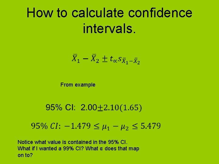
Confidence intervals • How was the 95% confidence interval calculated for the independent samples t test? – Make sure you know how to calculate for the test. – Make sure you know what value will be in or not in the interval. • If you reject the null with α =. 05 (zero will not be in 95% CI. • If you fail to reject the null with α =. 05 (zero will be in 95% CI).

How to calculate confidence intervals. From example Notice what value is contained in the 95% CI. What if I wanted a 99% CI? What α does that map on to?

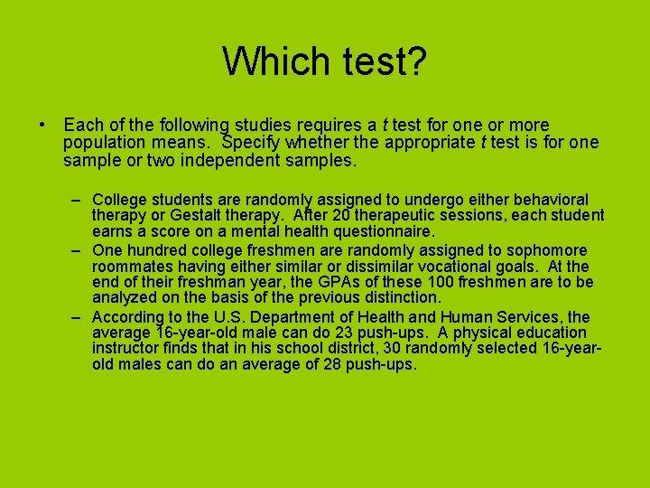
Which test? • Each of the following studies requires a t test for one or more population means. Specify whether the appropriate t test is for one sample or two independent samples. – College students are randomly assigned to undergo either behavioral therapy or Gestalt therapy. After 20 therapeutic sessions, each student earns a score on a mental health questionnaire. – One hundred college freshmen are randomly assigned to sophomore roommates having either similar or dissimilar vocational goals. At the end of their freshman year, the GPAs of these 100 freshmen are to be analyzed on the basis of the previous distinction. – According to the U. S. Department of Health and Human Services, the average 16 -year-old male can do 23 push-ups. A physical education instructor finds that in his school district, 30 randomly selected 16 -yearold males can do an average of 28 push-ups.

More on Statistical Significance Testing

The Problems with SST • We misunderstand what it does tell us. • It does not tell us what we want to know. • We often overemphasize SST.

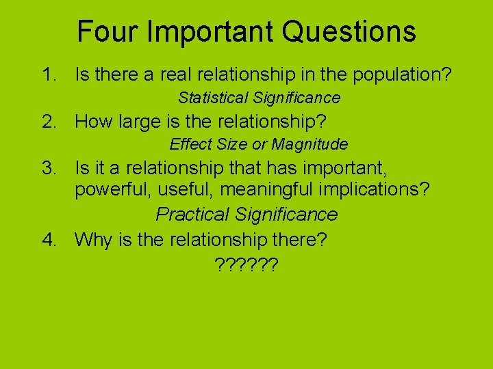
Four Important Questions 1. Is there a real relationship in the population? Statistical Significance 2. How large is the relationship? Effect Size or Magnitude 3. Is it a relationship that has important, powerful, useful, meaningful implications? Practical Significance 4. Why is the relationship there? ? ? ?

SST is all about. . . • Sampling Error – The difference between what I see in my sample and what exists in the target population. – Simply because I sampled, I could be wrong.

How it works: 1. Assume sampling error occurred; there is no difference in the population. 2. Build a statistical scenario based on this null hypothesis 3. How likely is it I got the sample value I got when the null hypothesis is true? (This is the p-value. )

How it works (cont’d): • How unlikely does my result have to be to rule out sampling error? alpha ( ). • If p < , then our result is statistically rare, is unlikely to occur when there isn’t a relationship in the population.

What it does tell us • Whether sampling error is a competing hypothesis for our finding.

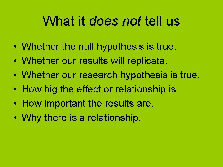
What it does not tell us • • • Whether the null hypothesis is true. Whether our results will replicate. Whether our research hypothesis is true. How big the effect or relationship is. How important the results are. Why there is a relationship.

Type I and II errors Power and Sample Size

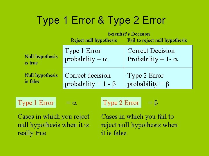
Type 1 Error & Type 2 Error Scientist’s Decision Reject null hypothesis Fail to reject null hypothesis Null hypothesis is true Null hypothesis is false Type 1 Error probability = Correct Decision Probability = 1 - Correct decision probability = 1 - Type 2 Error probability = = Cases in which you reject null hypothesis when it is really true Type 2 Error = Cases in which you fail to reject null hypothesis when it is false

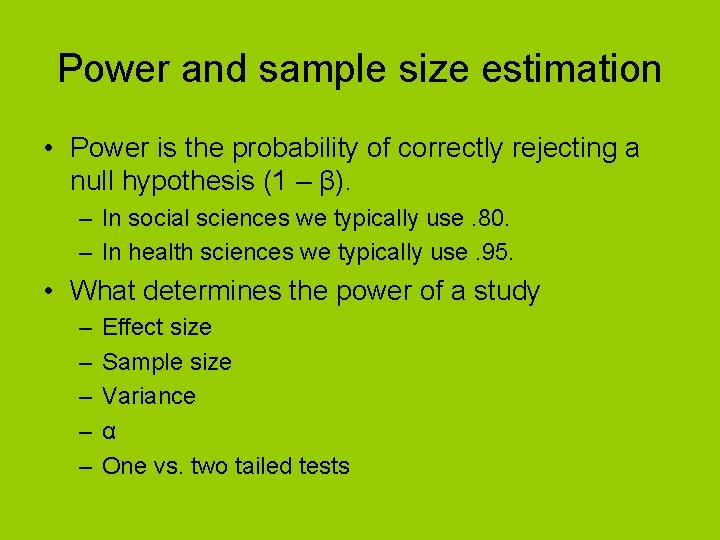
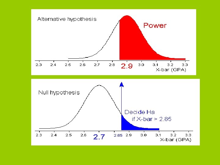
Power and sample size estimation • Power is the probability of correctly rejecting a null hypothesis (1 – β). – In social sciences we typically use. 80. – In health sciences we typically use. 95. • What determines the power of a study – – – Effect size Sample size Variance α One vs. two tailed tests

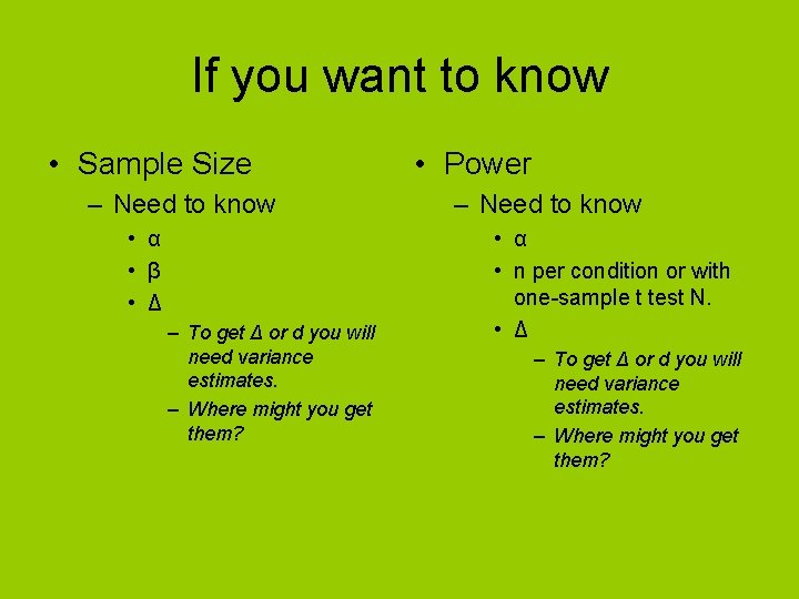
If you want to know • Sample Size – Need to know • α • β • Δ – To get Δ or d you will need variance estimates. – Where might you get them? • Power – Need to know • α • n per condition or with one-sample t test N. • Δ – To get Δ or d you will need variance estimates. – Where might you get them?

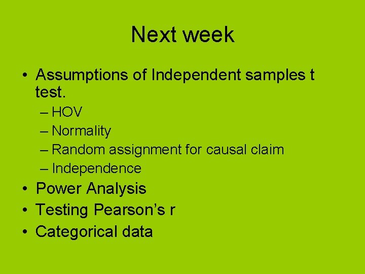
Next week • Assumptions of Independent samples t test. – HOV – Normality – Random assignment for causal claim – Independence • Power Analysis • Testing Pearson’s r • Categorical data