Dependence Precedence Precedence Dependence Can we execute a

Dependence Precedence

Precedence & Dependence • Can we execute a 1000 line program with 1000 processors in one step? • What are the issues to deal with in various parallelizing situations: – Parallel Programming? – Instruction Level Parallelism? • What type analysis is used to study concurrent database operation?

Dependence

Making Use of Processors • In parallelizing algorithms, we want to use as many processors as possible in an effort to finish in as little time as possible. • Often, it is not possible to make complete use of all processors in all time units – Some instructions (or sections of instructions) depend upon others – Others have a different, related problem called precedence (next section)

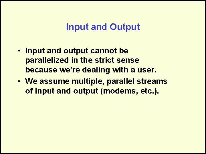
Input and Output • Input and output cannot be parallelized in the strict sense because we’re dealing with a user. • We assume multiple, parallel streams of input and output (modems, etc. ).

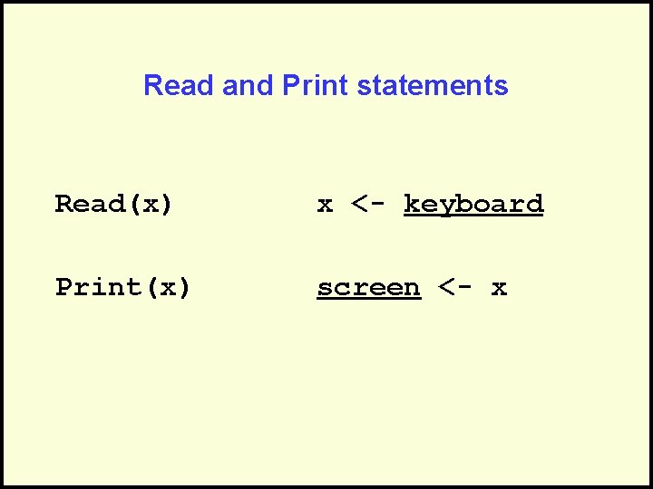
Read and Print statements Read(x) x <- keyboard Print(x) screen <- x

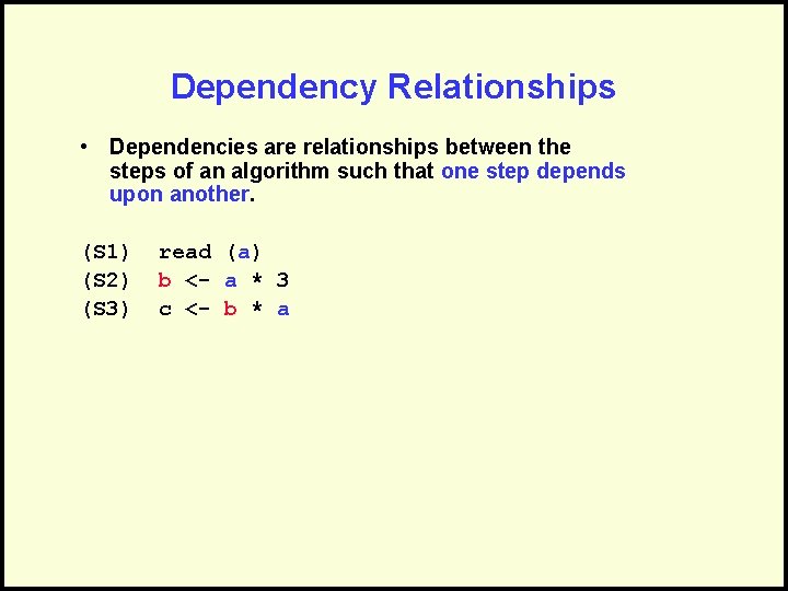
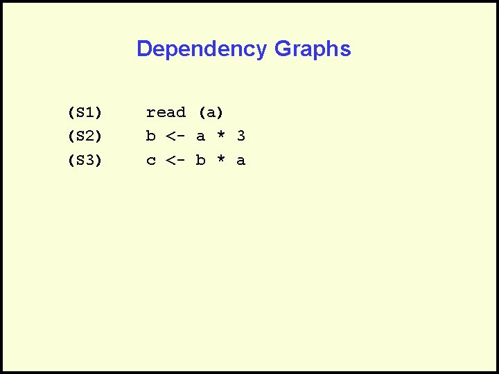
Dependency Relationships • Dependencies are relationships between the steps of an algorithm such that one step depends upon another. (S 1) (S 2) (S 3) read (a) b <- a * 3 c <- b * a

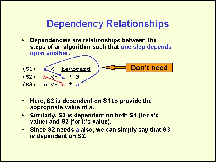
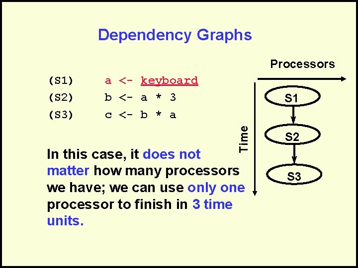
Dependency Relationships • Dependencies are relationships between the steps of an algorithm such that one step depends upon another. (S 1) (S 2) (S 3) a <- keyboard b <- a * 3 c <- b * a Don’t need • Here, S 2 is dependent on S 1 to provide the appropriate value of a. • Similarly, S 3 is dependent on both S 1 (for a’s value) and S 2 (for b’s value). • Since S 2 needs a also, we can simply say that S 3 is dependent on S 2.

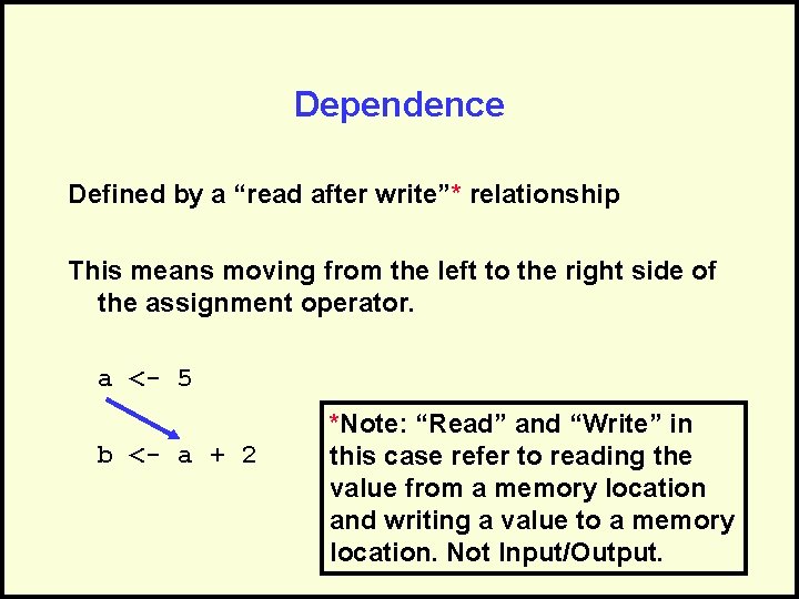
Dependence Defined by a “read after write”* relationship This means moving from the left to the right side of the assignment operator. a <- 5 b <- a + 2 *Note: “Read” and “Write” in this case refer to reading the value from a memory location and writing a value to a memory location. Not Input/Output.

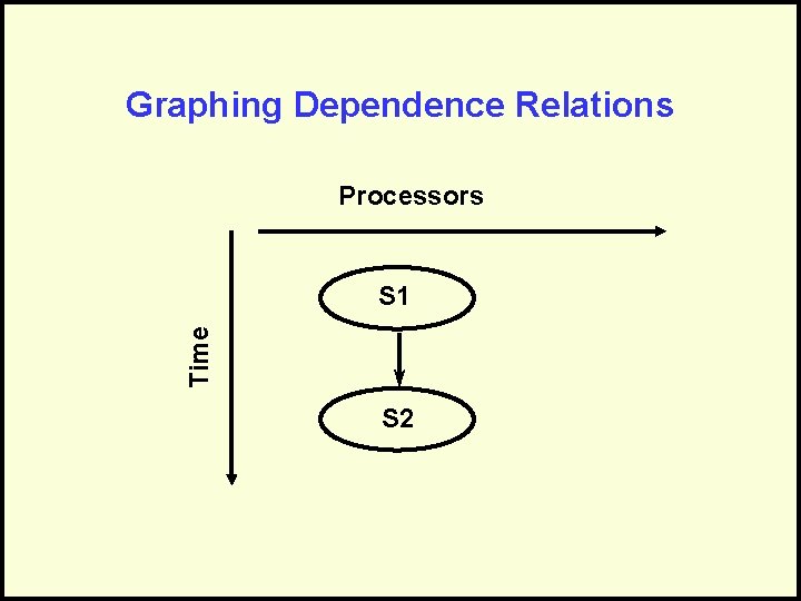
Graphing Dependence Relations Processors Time S 1 S 2

Dependency Graphs (S 1) (S 2) (S 3) read (a) b <- a * 3 c <- b * a

Dependency Graphs Processors a <- keyboard b <- a * 3 c <- b * a S 1 Time (S 1) (S 2) (S 3) In this case, it does not matter how many processors we have; we can use only one processor to finish in 3 time units. S 2 S 3

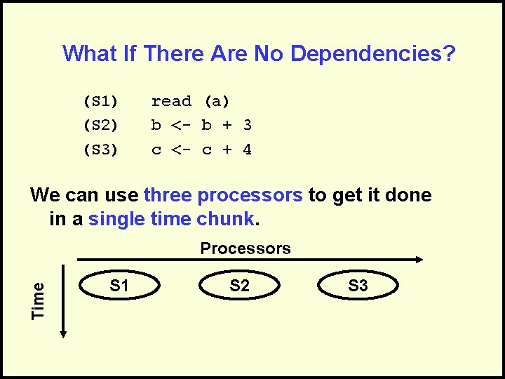
What If There Are No Dependencies? (S 1) (S 2) (S 3) read (a) b <- b + 3 c <- c + 4 We can use three processors to get it done in a single time chunk. Time Processors S 1 S 2 S 3

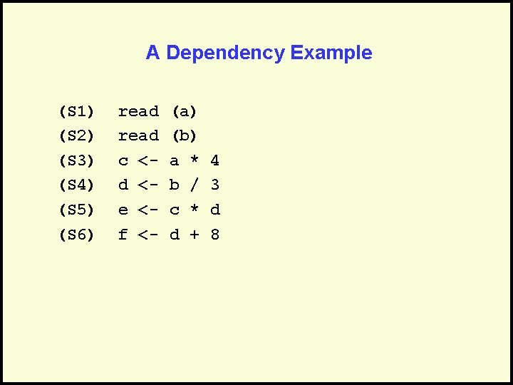
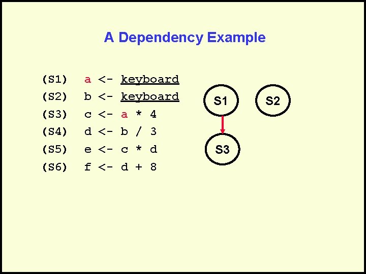
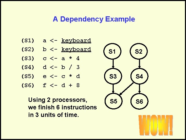
A Dependency Example (S 1) (S 2) (S 3) (S 4) (S 5) (S 6) read c <d <e <f <- (a) (b) a * b / c * d + 4 3 d 8

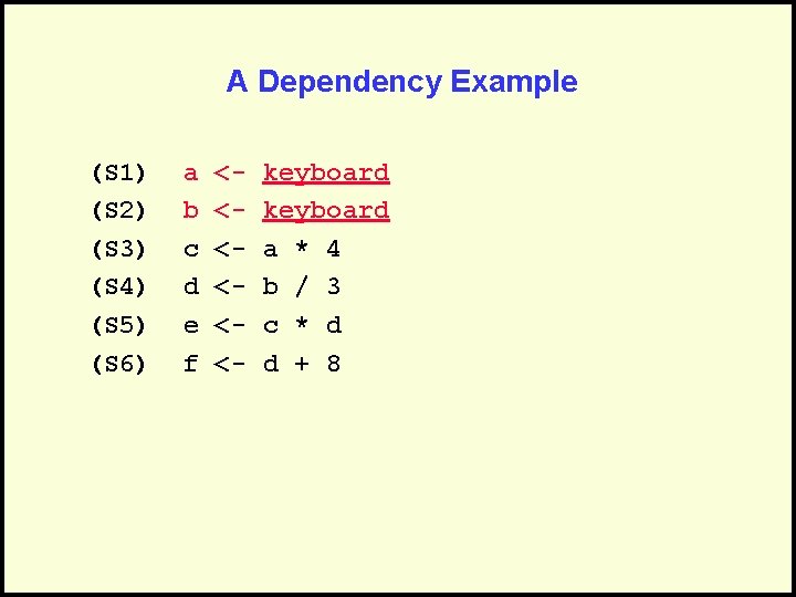
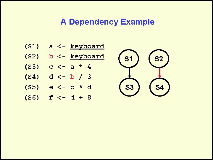
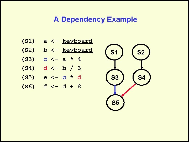
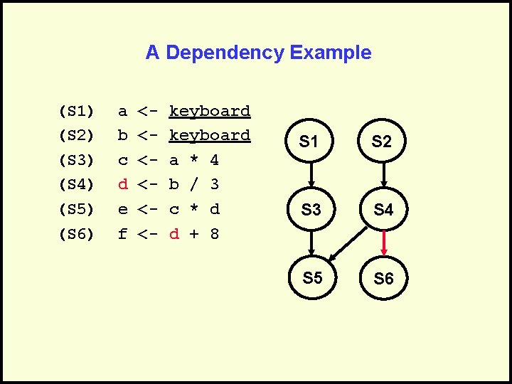
A Dependency Example (S 1) (S 2) (S 3) (S 4) (S 5) (S 6) a b c d e f <<<<<<- keyboard a * 4 b / 3 c * d d + 8

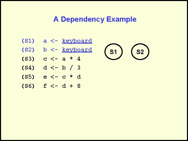
A Dependency Example (S 1) (S 2) (S 3) (S 4) (S 5) (S 6) a b c d e f <<<<<<- keyboard a * 4 b / 3 c * d d + 8 S 1 S 2

A Dependency Example (S 1) (S 2) (S 3) (S 4) (S 5) (S 6) a b c d e f <<<<<<- keyboard a * 4 b / 3 c * d d + 8 S 1 S 3 S 2

A Dependency Example (S 1) (S 2) (S 3) (S 4) (S 5) (S 6) a b c d e f <<<<<<- keyboard a * 4 b / 3 c * d d + 8 S 1 S 2 S 3 S 4

A Dependency Example (S 1) (S 2) (S 3) (S 4) (S 5) (S 6) a b c d e f <<<<<<- keyboard a * 4 b / 3 c * d d + 8 S 1 S 2 S 3 S 4 S 5

A Dependency Example (S 1) (S 2) (S 3) (S 4) (S 5) (S 6) a b c d e f <<<<<<- keyboard a * 4 b / 3 c * d d + 8 S 1 S 2 S 3 S 4 S 5 S 6

A Dependency Example (S 1) (S 2) (S 3) (S 4) (S 5) (S 6) a b c d e f <<<<<<- keyboard a * 4 b / 3 c * d d + 8 Using 2 processors, we finish 6 instructions in 3 units of time. S 1 S 2 S 3 S 4 S 5 S 6

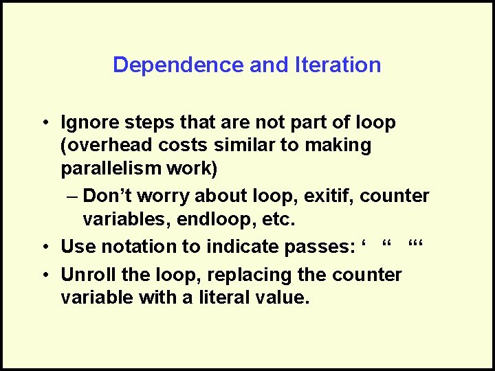
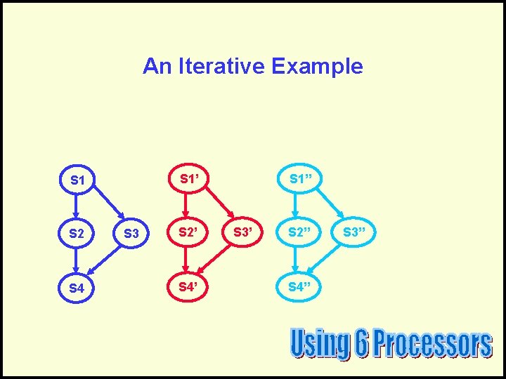
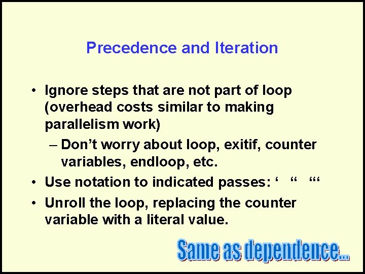
Dependence and Iteration • Ignore steps that are not part of loop (overhead costs similar to making parallelism work) – Don’t worry about loop, exitif, counter variables, endloop, etc. • Use notation to indicate passes: ‘ “ “‘ • Unroll the loop, replacing the counter variable with a literal value.

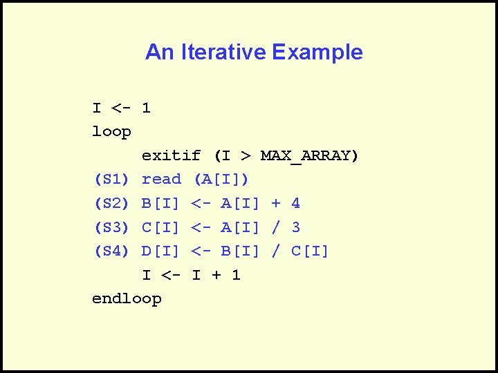
An Iterative Example I <- 1 loop exitif (I > MAX_ARRAY) (S 1) read (A[I]) (S 2) B[I] <- A[I] + 4 (S 3) C[I] <- A[I] / 3 (S 4) D[I] <- B[I] / C[I] I <- I + 1 endloop

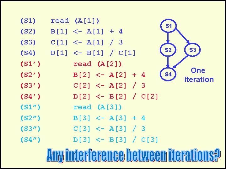
(S 1) (S 2) (S 3) (S 4) (S 1’) (S 2’) (S 3’) (S 4’) (S 1”) (S 2”) (S 3”) (S 4”) read B[1] C[1] D[1] (A[1]) <- A[1] + 4 <- A[1] / 3 <- B[1] / C[1] read (A[2]) B[2] <- A[2] + C[2] <- A[2] / D[2] <- B[2] / read (A[3]) B[3] <- A[3] + C[3] <- A[3] / D[3] <- B[3] / S 1 S 2 4 3 C[2] 4 3 C[3] S 4 S 3 One iteration

An Iterative Example S 1’ S 1 S 2 S 4 S 3 S 2’ S 4’ S 1” S 3’ S 2” S 4” S 3”

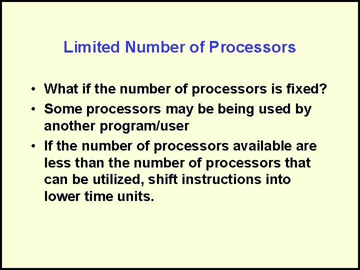
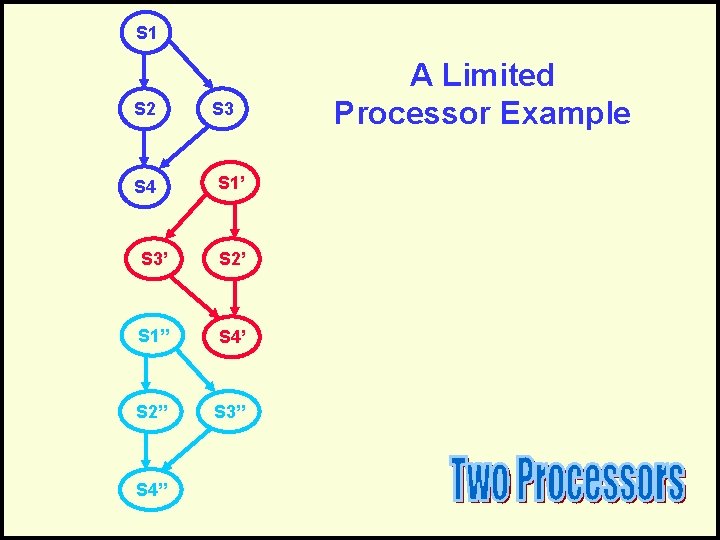
Limited Number of Processors • What if the number of processors is fixed? • Some processors may be being used by another program/user • If the number of processors available are less than the number of processors that can be utilized, shift instructions into lower time units.

S 1 S 2 S 4 S 3 S 1’ S 3’ S 2’ S 1” S 4’ S 2” S 3” S 4” A Limited Processor Example

Questions?

Precedence

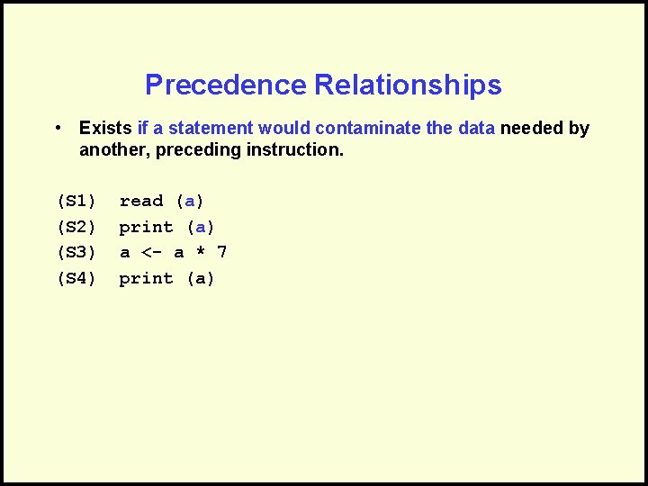
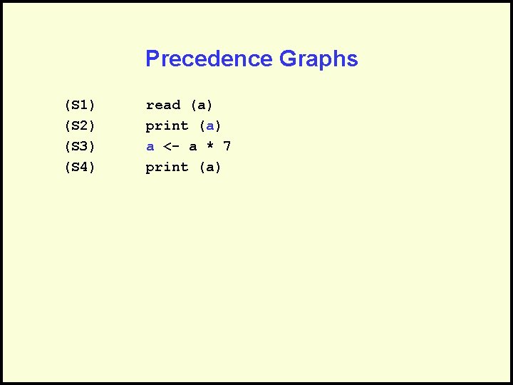
Precedence Relationships • Exists if a statement would contaminate the data needed by another, preceding instruction. (S 1) (S 2) (S 3) (S 4) read (a) print (a) a <- a * 7 print (a)

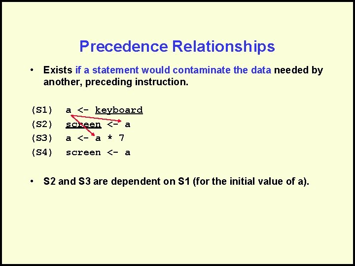
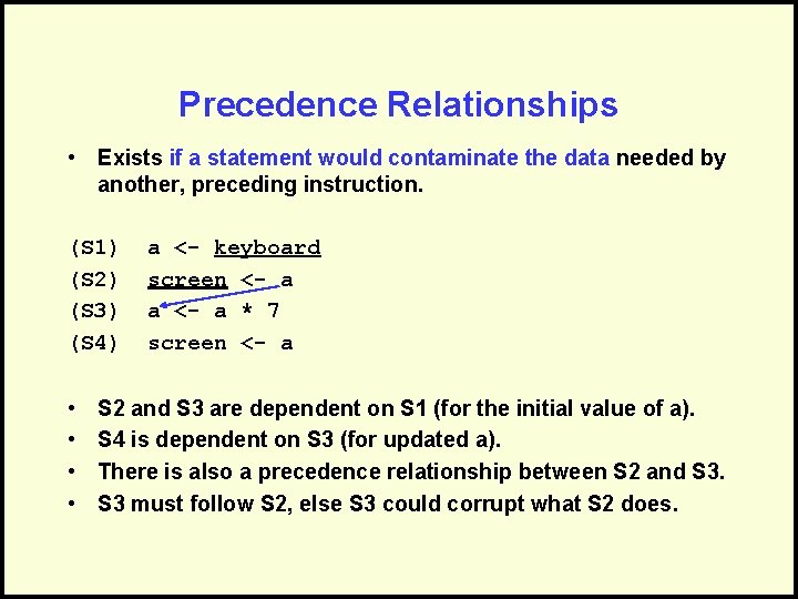
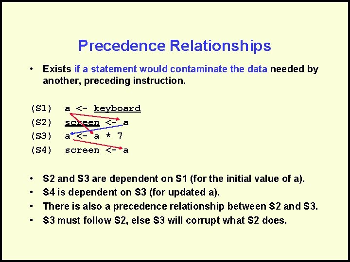
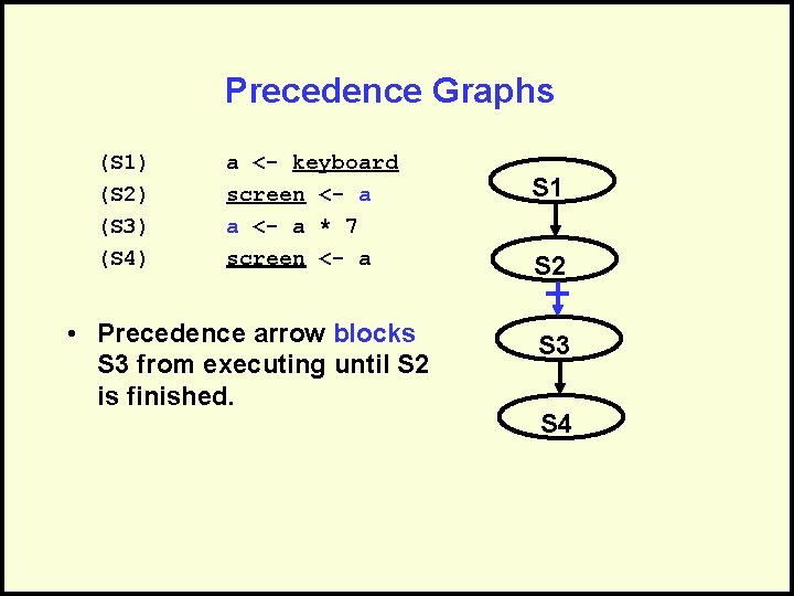
Precedence Relationships • Exists if a statement would contaminate the data needed by another, preceding instruction. (S 1) (S 2) (S 3) (S 4) a <- keyboard screen <- a a <- a * 7 screen <- a • S 2 and S 3 are dependent on S 1 (for the initial value of a).

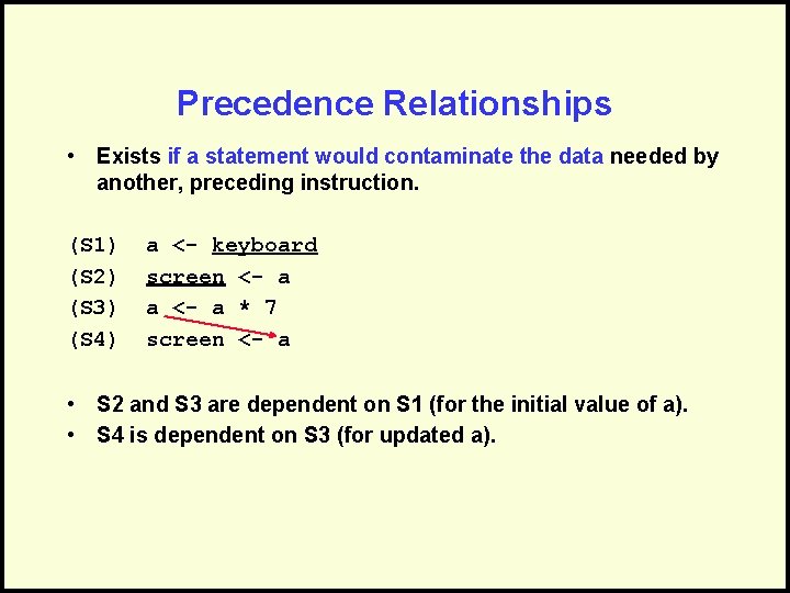
Precedence Relationships • Exists if a statement would contaminate the data needed by another, preceding instruction. (S 1) (S 2) (S 3) (S 4) a <- keyboard screen <- a a <- a * 7 screen <- a • S 2 and S 3 are dependent on S 1 (for the initial value of a). • S 4 is dependent on S 3 (for updated a).

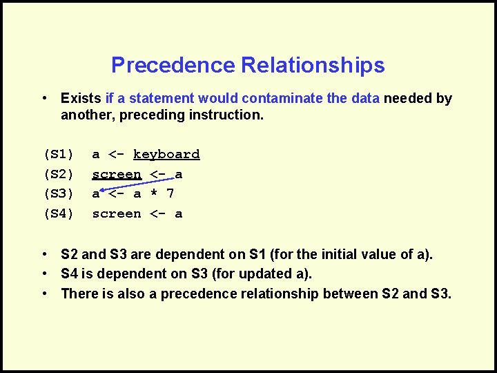
Precedence Relationships • Exists if a statement would contaminate the data needed by another, preceding instruction. (S 1) (S 2) (S 3) (S 4) a <- keyboard screen <- a a <- a * 7 screen <- a • S 2 and S 3 are dependent on S 1 (for the initial value of a). • S 4 is dependent on S 3 (for updated a). • There is also a precedence relationship between S 2 and S 3.

Precedence Relationships • Exists if a statement would contaminate the data needed by another, preceding instruction. (S 1) (S 2) (S 3) (S 4) • • a <- keyboard screen <- a a <- a * 7 screen <- a S 2 and S 3 are dependent on S 1 (for the initial value of a). S 4 is dependent on S 3 (for updated a). There is also a precedence relationship between S 2 and S 3 must follow S 2, else S 3 could corrupt what S 2 does.

Precedence Relationships • Exists if a statement would contaminate the data needed by another, preceding instruction. (S 1) (S 2) (S 3) (S 4) • • a <- keyboard screen <- a a <- a * 7 screen <- a S 2 and S 3 are dependent on S 1 (for the initial value of a). S 4 is dependent on S 3 (for updated a). There is also a precedence relationship between S 2 and S 3 must follow S 2, else S 3 will corrupt what S 2 does.

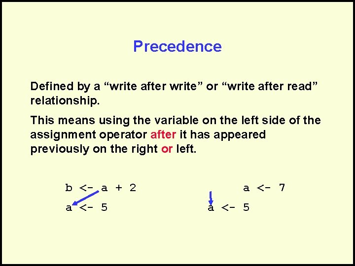
Precedence Defined by a “write after write” or “write after read” relationship. This means using the variable on the left side of the assignment operator after it has appeared previously on the right or left. b <- a + 2 a <- 5 a <- 7 a <- 5

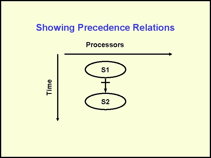
Showing Precedence Relations Processors Time S 1 S 2

Precedence Graphs (S 1) (S 2) (S 3) (S 4) read (a) print (a) a <- a * 7 print (a)

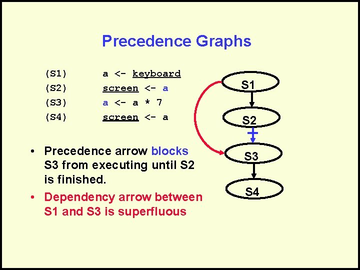
Precedence Graphs (S 1) (S 2) (S 3) (S 4) a <- keyboard screen <- a a <- a * 7 screen <- a • Precedence arrow blocks S 3 from executing until S 2 is finished. S 1 S 2 S 3 S 4

Precedence Graphs (S 1) (S 2) (S 3) (S 4) a <- keyboard screen <- a a <- a * 7 screen <- a • Precedence arrow blocks S 3 from executing until S 2 is finished. • Dependency arrow between S 1 and S 3 is superfluous S 1 S 2 S 3 S 4

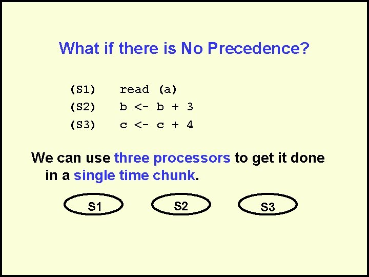
What if there is No Precedence? (S 1) (S 2) (S 3) read (a) b <- b + 3 c <- c + 4 We can use three processors to get it done in a single time chunk. S 1 S 2 S 3

Precedence and Iteration • Ignore steps that are not part of loop (overhead costs similar to making parallelism work) – Don’t worry about loop, exitif, counter variables, endloop, etc. • Use notation to indicated passes: ‘ “ “‘ • Unroll the loop, replacing the counter variable with a literal value.

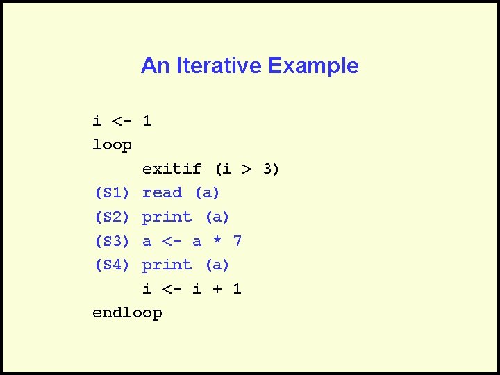
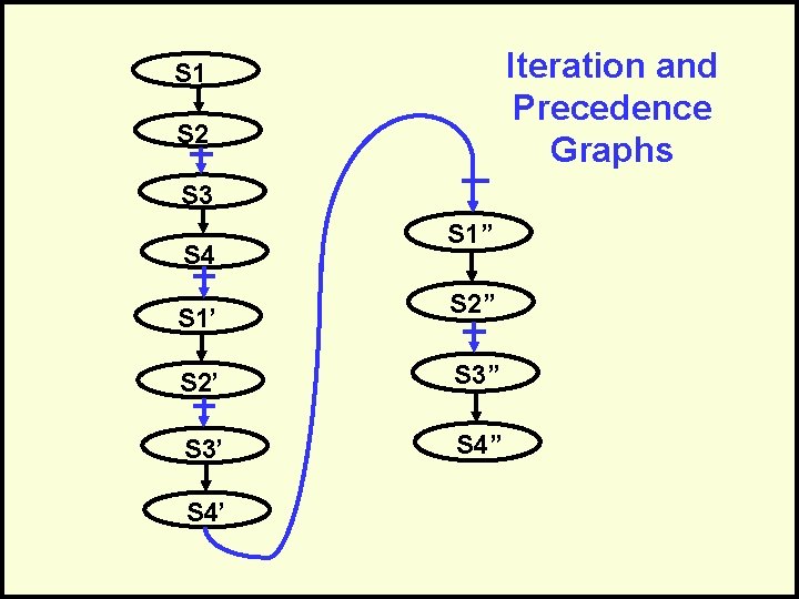
An Iterative Example i <- 1 loop exitif (i > 3) (S 1) read (a) (S 2) print (a) (S 3) a <- a * 7 (S 4) print (a) i <- i + 1 endloop

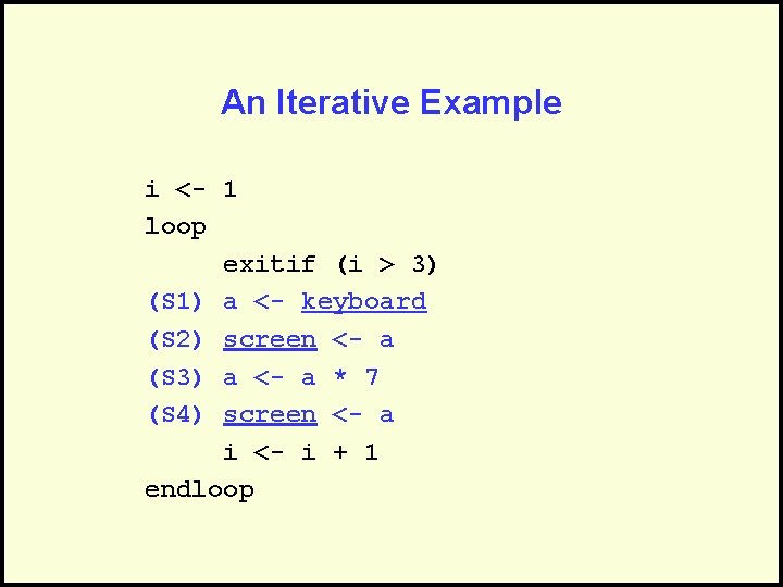
An Iterative Example i <- 1 loop exitif (i > 3) (S 1) a <- keyboard (S 2) screen <- a (S 3) a <- a * 7 (S 4) screen <- a i <- i + 1 endloop

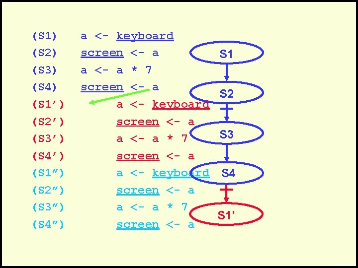
(S 1) (S 2) (S 3) (S 4) (S 1’) (S 2’) (S 3’) (S 4’) (S 1”) (S 2”) (S 3”) (S 4”) a <- keyboard screen <- a a <- a * 7 screen <- a S 1 S 2 S 3 S 4 S 1’

Iteration and Precedence Graphs S 1 S 2 S 3 S 4 S 1’ S 1” S 2’ S 3” S 3’ S 4” S 4’

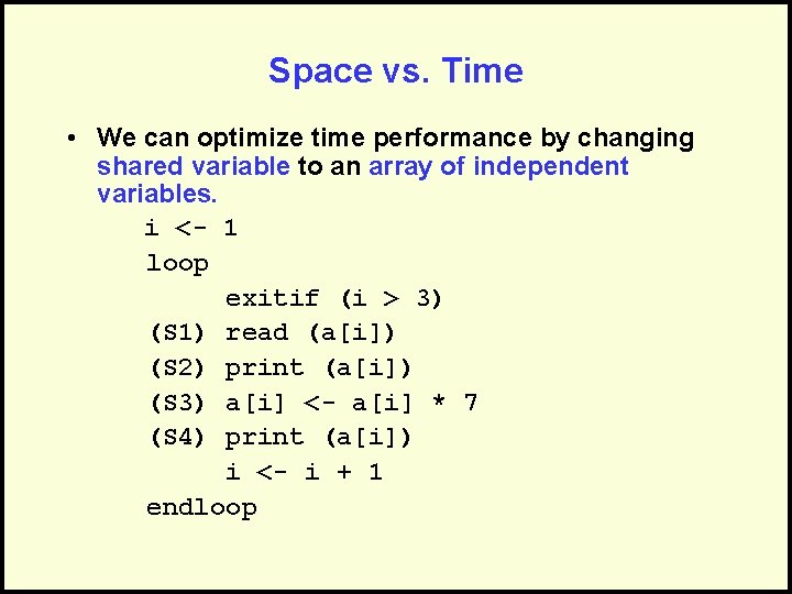
Space vs. Time • We can optimize time performance by changing shared variable to an array of independent variables. i <- 1 loop exitif (i > 3) (S 1) read (a[i]) (S 2) print (a[i]) (S 3) a[i] <- a[i] * 7 (S 4) print (a[i]) i <- i + 1 endloop

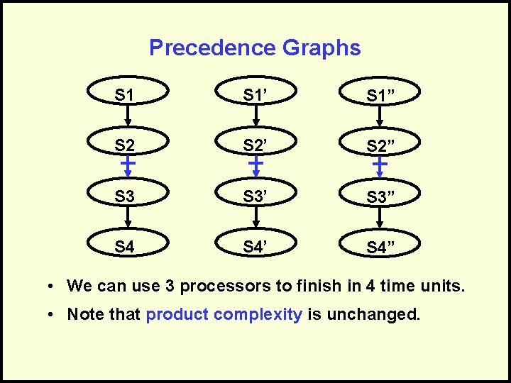
Precedence Graphs S 1’ S 1” S 2’ S 2” S 3’ S 3” S 4’ S 4” • We can use 3 processors to finish in 4 time units. • Note that product complexity is unchanged.

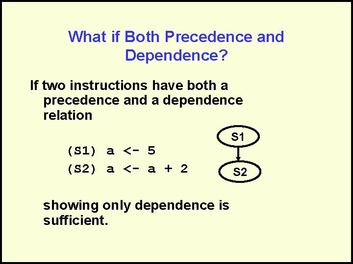
What if Both Precedence and Dependence? If two instructions have both a precedence and a dependence relation (S 1) a <- 5 (S 2) a <- a + 2 showing only dependence is sufficient. S 1 S 2

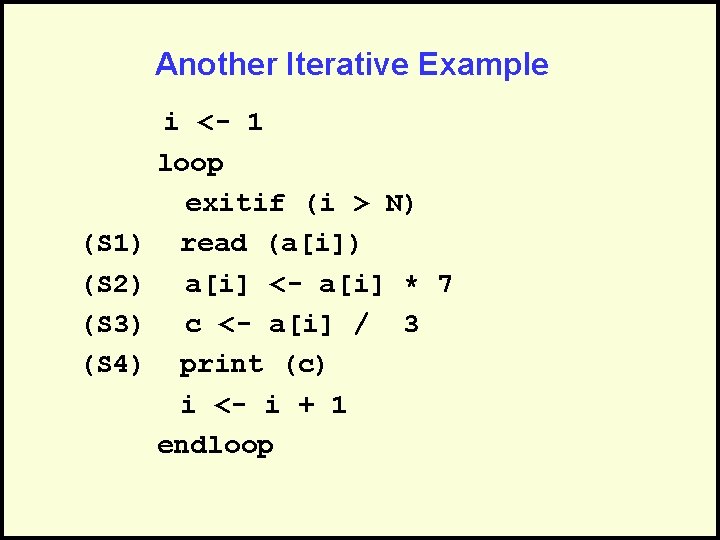
Another Iterative Example (S 1) (S 2) (S 3) (S 4) i <- 1 loop exitif (i > N) read (a[i]) a[i] <- a[i] * 7 c <- a[i] / 3 print (c) i <- i + 1 endloop

Another Iterative Example i <- 1 loop exitif (i > N) (S 1) a[i] <- keyboard (S 2) a[i] <- a[i] * 7 (S 3) c <- a[i] / 3 (S 4) screen <- c i <- i + 1 endloop

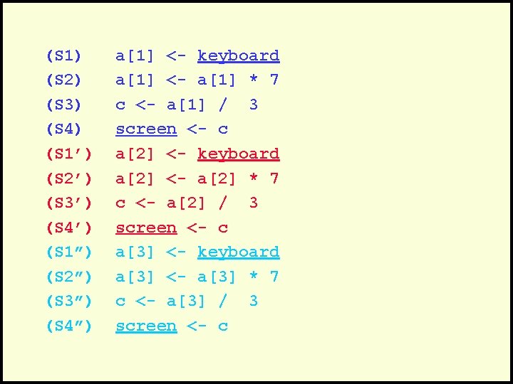
(S 1) (S 2) (S 3) (S 4) (S 1’) (S 2’) (S 3’) (S 4’) (S 1”) (S 2”) (S 3”) (S 4”) a[1] <- keyboard a[1] <- a[1] * 7 c <- a[1] / 3 screen <- c a[2] <- keyboard a[2] <- a[2] * 7 c <- a[2] / 3 screen <- c a[3] <- keyboard a[3] <- a[3] * 7 c <- a[3] / 3 screen <- c

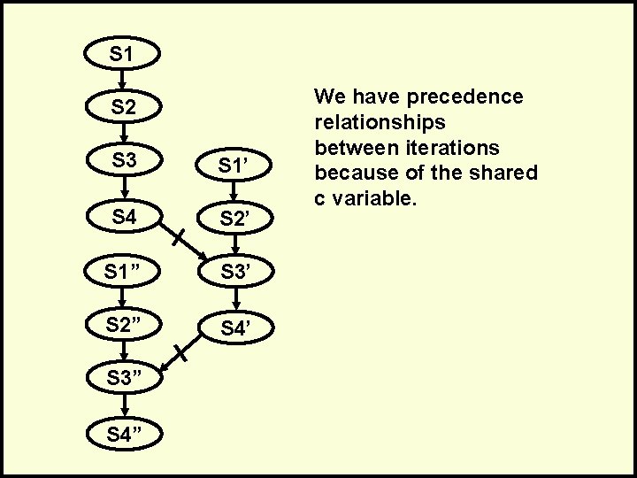
S 1 S 2 S 3 S 1’ S 4 S 2’ S 1” S 3’ S 2” S 4’ S 3” S 4” We have precedence relationships between iterations because of the shared c variable.

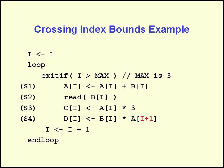
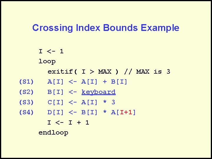
Crossing Index Bounds Example I <- 1 loop exitif( I > MAX ) (S 1) A[I] <- A[I] (S 2) read( B[I] ) (S 3) C[I] <- A[I] (S 4) D[I] <- B[I] I <- I + 1 endloop // MAX is 3 + B[I] * 3 * A[I+1]

Crossing Index Bounds Example (S 1) (S 2) (S 3) (S 4) I <- 1 loop exitif( I > MAX ) // MAX is 3 A[I] <- A[I] + B[I] <- keyboard C[I] <- A[I] * 3 D[I] <- B[I] * A[I+1] I <- I + 1 endloop

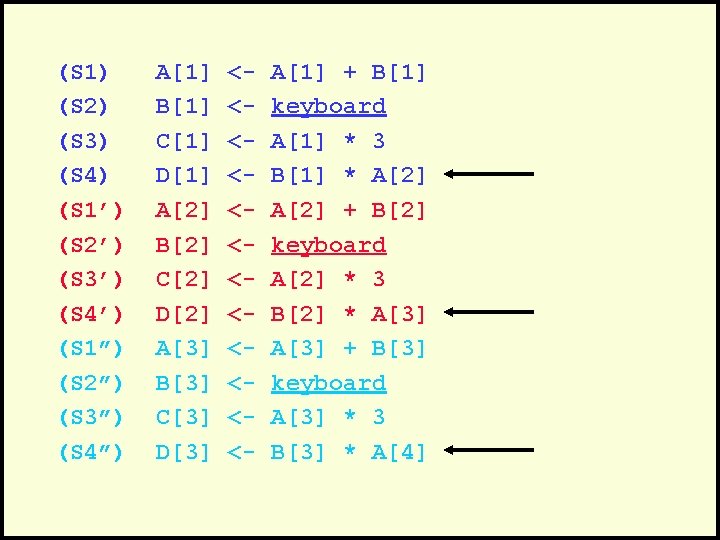
(S 1) (S 2) (S 3) (S 4) (S 1’) (S 2’) (S 3’) (S 4’) (S 1”) (S 2”) (S 3”) (S 4”) A[1] B[1] C[1] D[1] A[2] B[2] C[2] D[2] A[3] B[3] C[3] D[3] <<<<<<- A[1] + B[1] keyboard A[1] * 3 B[1] * A[2] + B[2] keyboard A[2] * 3 B[2] * A[3] + B[3] keyboard A[3] * 3 B[3] * A[4]

S 1 S 2 S 3 S 4 S 1’ S 2’ S 4’ S 3’ Precedence between iterations

Questions?

Practical Applications • We used the single assignments as easy illustrations of the principles. • There additional real applications of this capability: – Much bigger than one assignment – Smaller than one assignment

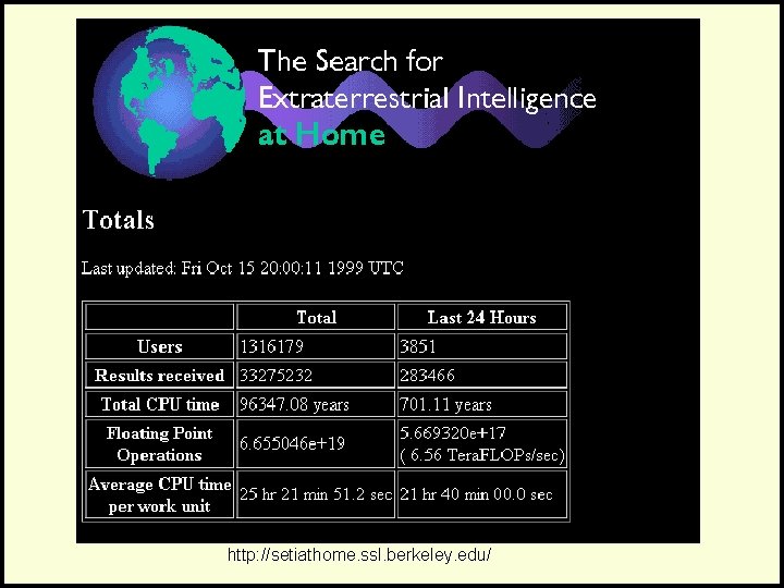
http: //setiathome. ssl. berkeley. edu/

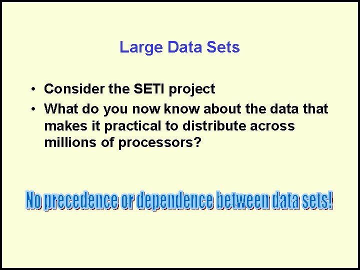
Large Data Sets • Consider the SETI project • What do you now know about the data that makes it practical to distribute across millions of processors?

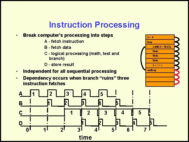
Instruction Processing • Break computer’s processing into steps I <- 0 A - fetch instruction B - fetch data C - logical processing (math, test and branch) D - store result • • loop exitif( I > MAX) blah. . . I <- I + 1 Independent for all sequential processing Dependency occurs when branch “ruins” three instruction fetches A 2 1 B 3 4 2 1 C 5 3 0 1 2 3 2 time 4 5 4 3 1 D 5 4 2 1 endloop 5 5 4 3 6 7

Questions?