DEPARTMENT OF QUANTITATIVE METHODS INFORMATION SYSTEMS Introduction to
- Slides: 42

DEPARTMENT OF QUANTITATIVE METHODS & INFORMATION SYSTEMS Introduction to Business Statistics QM 120 Chapter 6

Continuous Probability Distribution 2 When a RV x is discrete, we can assign a positive probability to each value that x can take and get the probability distribution for x. Ø Ø The sum of all probabilities of all values of x is 1. Ø Not all experiments result in RVs that are discrete. Continuous RV, such as heights, weights, lifetime of a particular product, experimental laboratory error…etc. can assume infinitely many values corresponding to points on line interval. Ø

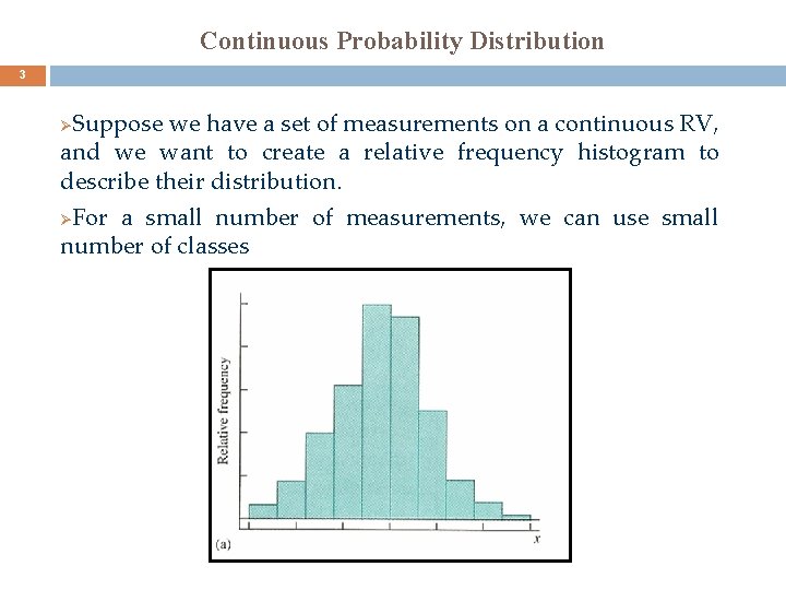
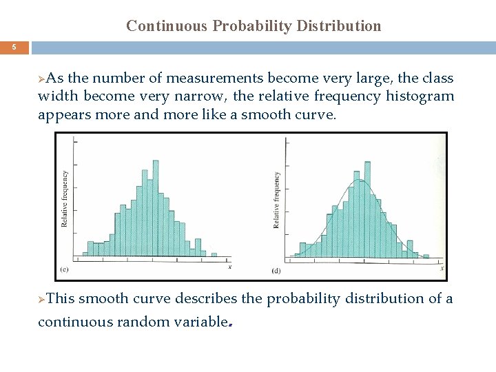
Continuous Probability Distribution 3 Suppose we have a set of measurements on a continuous RV, and we want to create a relative frequency histogram to describe their distribution. Ø For a small number of measurements, we can use small number of classes Ø

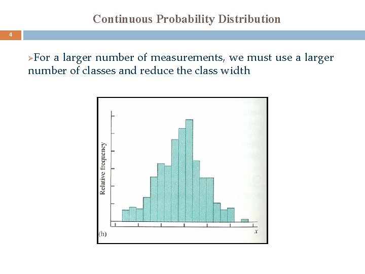
Continuous Probability Distribution 4 For a larger number of measurements, we must use a larger number of classes and reduce the class width Ø

Continuous Probability Distribution 5 As the number of measurements become very large, the class width become very narrow, the relative frequency histogram appears more and more like a smooth curve. Ø Ø This smooth curve describes the probability distribution of a continuous random variable.

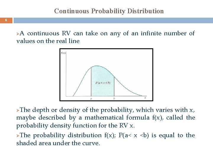
Continuous Probability Distribution 6 A continuous RV can take on any of an infinite number of values on the real line Ø The depth or density of the probability, which varies with x, maybe described by a mathematical formula f(x), called the probability density function for the RV x. Ø The probability distribution f(x); P(a< x <b) is equal to the shaded area under the curve. Ø

Continuous Probability Distribution 7 Several important properties of continuous probability distribution parallel their discrete part. Ø Ø Just as the sum of discrete probabilities is equal to 1, i. e. P(x) = 1, and the probability that x falls into a certain interval can be found by summing the probabilities in that interval, continuous probability distributions have the following two characteristics: Ø Ø The area under a continuous probability distribution is equal to 1. The probability that x will fall into a particular interval- say, from a to b – is equal to the area under the curve between the two points a and b

Continuous Probability Distribution 8 There is a very important difference between the continuous case and the discrete one which is: Ø Ø P(x = a) = 0 Ø P(a < x < b) = P(a ≤ x ≤ b) Ø P( x < a) = P( x ≤ a)

The Normal Distribution 9 Among many continuous probability distributions, the normal distribution is the most important and widely used one. Ø Ø A large number of real world phenomena are either exactly or approximately normally distributed. The normal distribution or Gaussian distribution is given by a bell-shaped curve. Ø A continuous RV x that has a normal distribution is said to be a normal RV with a mean and a standard deviation or simply x~N( , ). Ø Note that not all the bell-shaped curves represent a normal distribution. Ø

The Normal Distribution 10 The normal probability distribution, when plotted, gives a bell -shaped curve such that Ø Ø The total area under the curve is 1. 0. Ø The curve is symmetric around the mean. Ø The two tails of the curve extended indefinitely. The mean and the standard deviation are the parameters of the normal distribution. Ø Given the values of these two parameters, we can find the area under the normal curve for any interval. Ø

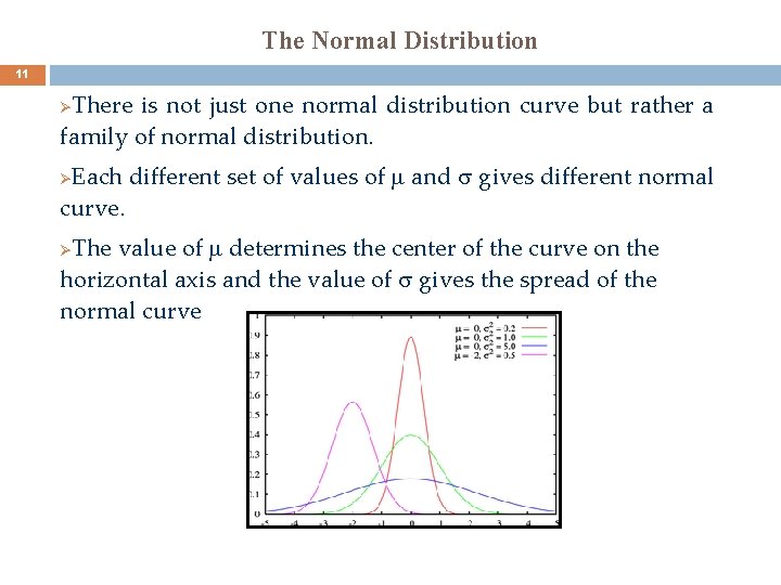
The Normal Distribution 11 There is not just one normal distribution curve but rather a family of normal distribution. Ø Each different set of values of and gives different normal curve. Ø The value of determines the center of the curve on the horizontal axis and the value of gives the spread of the normal curve Ø

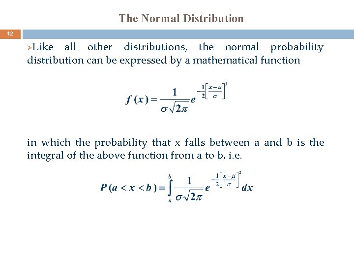
The Normal Distribution 12 Like all other distributions, the normal probability distribution can be expressed by a mathematical function Ø in which the probability that x falls between a and b is the integral of the above function from a to b, i. e.

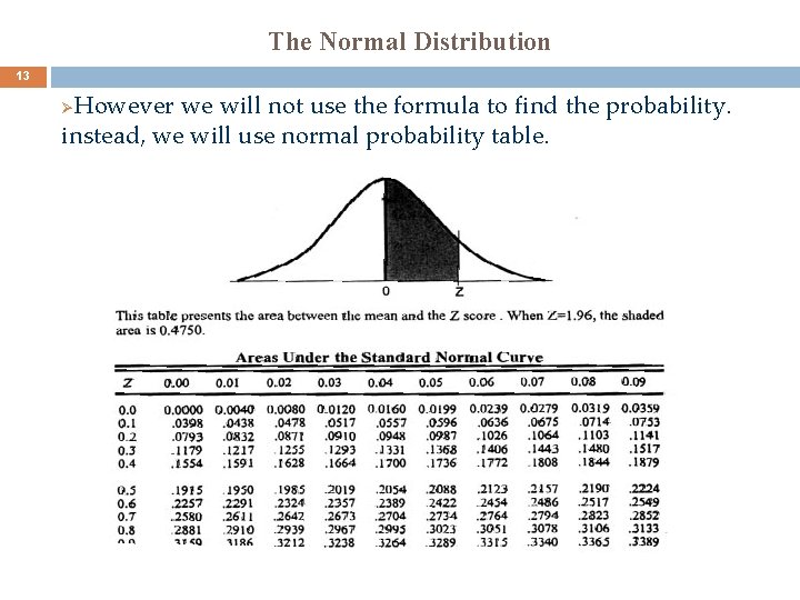
The Normal Distribution 13 However we will not use the formula to find the probability. instead, we will use normal probability table. Ø

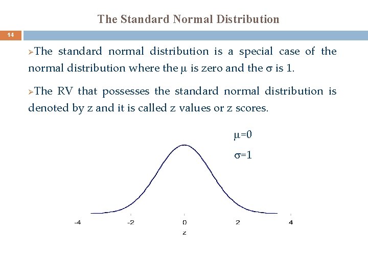
The Standard Normal Distribution 14 The standard normal distribution is a special case of the normal distribution where the is zero and the is 1. Ø Ø The RV that possesses the standard normal distribution is denoted by z and it is called z values or z scores. =0 =1

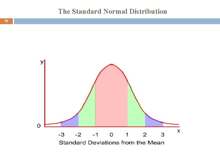
The Standard Normal Distribution 15 Since is zero and the is 1 for the standard normal, a specific value of z gives the distance between the mean and the point represented by z in terms of the standard deviation. Ø The z values to the right side of the mean are positive and those on the left are negative BUT the area under the curve is always positive. Ø For a value of z = 2, we are 2 standard deviations from the mean (to the right). Ø Similarly, for z = -2, we are 2 standard deviations from the mean (to the left) Ø

The Standard Normal Distribution 16

The Standard Normal Distribution 17 The standard normal table lists the area under the standard normal curve between z = 0 to the values of z to 3. 09. Ø Ø To read the standard normal table, we always start at z = 0, which represents the mean. Always remember that the normal curve is symmetric, that is the area from 0 to any positive z value is equal to the area from 0 to that value in the negative side. Ø

The Standard Normal Distribution 18 Example: Find the area under the standard normal curve between z = 0 to z = 1. 95 Example: Find the area under the standard normal curve between z = -2. 17 to z = 0

The Standard Normal Distribution 19 Example: Find the following areas under the standard normal curve. a) Area to the right of z = 2. 32 b) Area to the left of z = -1. 54

The Standard Normal Distribution 20 Example: Find the following probabilities for the standard normal curve. a) P(1. 19 < z < 2. 12) b) P(-1. 56 < z < 2. 31) c) P(z > -. 75)

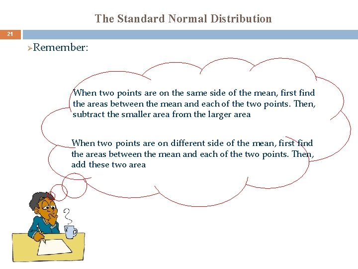
The Standard Normal Distribution 21 Ø Remember: When two points are on the same side of the mean, first find the areas between the mean and each of the two points. Then, subtract the smaller area from the larger area When two points are on different side of the mean, first find the areas between the mean and each of the two points. Then, add these two area

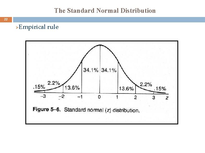
The Standard Normal Distribution 22 Ø Empirical rule

The Standard Normal Distribution 23 Example: Find the following probabilities for the standard normal curve. a) P(0 < z < 5. 65) b) P( z < - 5. 3)

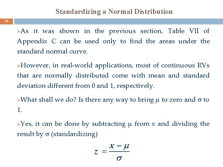
Standardizing a Normal Distribution 24 As it was shown in the previous section, Table VII of Appendix C can be used only to find the areas under the standard normal curve. Ø However, in real-world applications, most of continuous RVs that are normally distributed come with mean and standard deviation different from 0 and 1, respectively. Ø What shall we do? Is there any way to bring to zero and to 1. Ø Yes, it can be done by subtracting from x and dividing the result by (standardizing) Ø

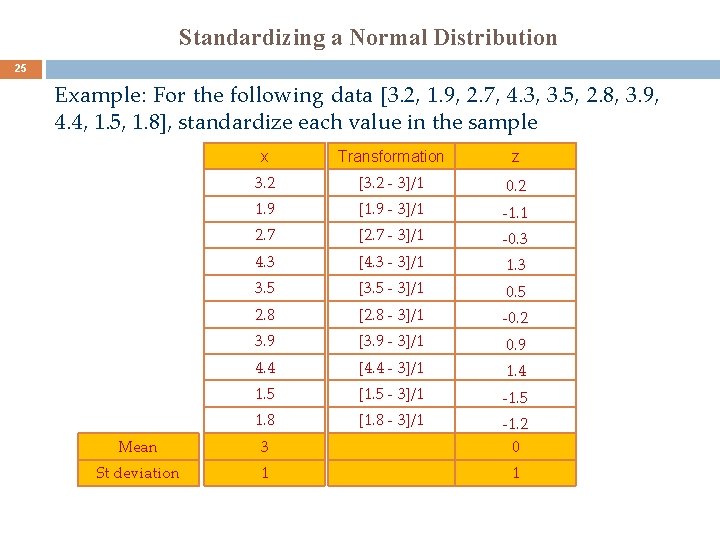
Standardizing a Normal Distribution 25 Example: For the following data [3. 2, 1. 9, 2. 7, 4. 3, 3. 5, 2. 8, 3. 9, 4. 4, 1. 5, 1. 8], standardize each value in the sample x Transformation z 3. 2 [3. 2 - 3]/1 0. 2 1. 9 [1. 9 - 3]/1 -1. 1 2. 7 [2. 7 - 3]/1 -0. 3 4. 3 [4. 3 - 3]/1 1. 3 3. 5 [3. 5 - 3]/1 0. 5 2. 8 [2. 8 - 3]/1 -0. 2 3. 9 [3. 9 - 3]/1 0. 9 4. 4 [4. 4 - 3]/1 1. 4 1. 5 [1. 5 - 3]/1 -1. 5 1. 8 [1. 8 - 3]/1 Mean 3 -1. 2 0 St deviation 1 1

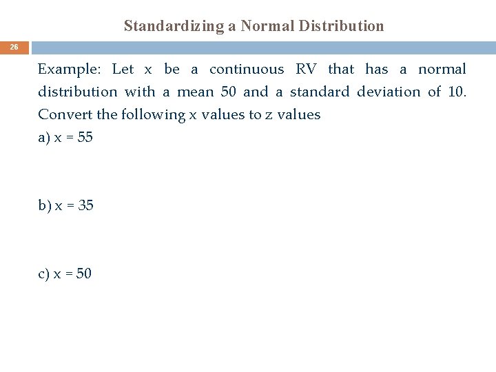
Standardizing a Normal Distribution 26 Example: Let x be a continuous RV that has a normal distribution with a mean 50 and a standard deviation of 10. Convert the following x values to z values a) x = 55 b) x = 35 c) x = 50

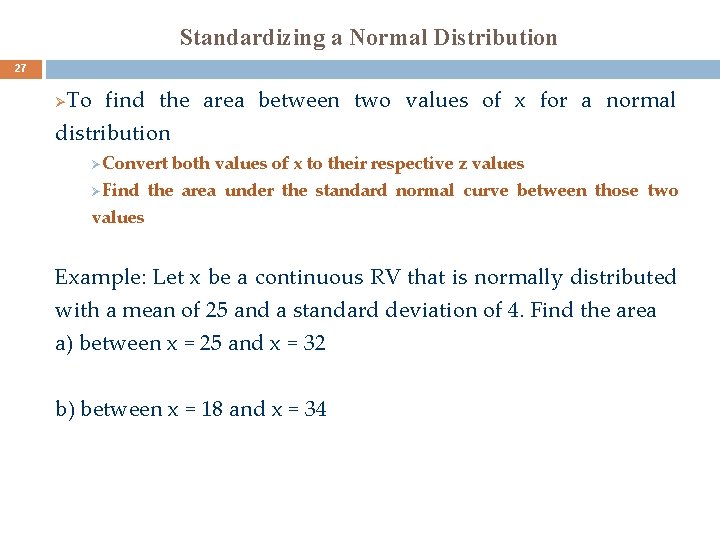
Standardizing a Normal Distribution 27 To find the area between two values of x for a normal distribution Ø ØConvert both values of x to their respective z values ØFind the area under the standard normal curve between those two values Example: Let x be a continuous RV that is normally distributed with a mean of 25 and a standard deviation of 4. Find the area a) between x = 25 and x = 32 b) between x = 18 and x = 34

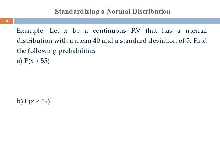
Standardizing a Normal Distribution 28 Example: Let x be a continuous RV that has a normal distribution with a mean 40 and a standard deviation of 5. Find the following probabilities a) P(x > 55) b) P(x < 49)

Standardizing a Normal Distribution 29 Example: Let x be a continuous RV that has a normal distribution with a mean 50 and a standard deviation of 8. Find the probability P(30 < x < 39)

Standardizing a Normal Distribution 30 Example: Let x be a continuous RV that has a normal distribution with a mean 80 and a standard deviation of 12. Find the following probabilities a) P(70 <x < 135) b) P(x < 27)

Application of the Normal Distribution 31 Example: According to the U. S. Bureau of Census, the mean income of all U. S. families was $43, 237 in 1991. Assume that the 1991 incomes of all U. S. families have a normal distribution with a mean of $43, 237 and a standard deviation of $10, 500. Find the probability that the 1991 income of a randomly selected U. S. family was between $30, 000 and $50, 000.

Application of the Normal Distribution 32 Example: A racing car is one of the many toys manufactured by Mack Corporation. The assembly time for this toy follows a normal distribution with a mean of 55 minutes and a standard deviation of 4 minutes. The company closes at 5 P. M. every day. If one worker starts assembling a racing car at 4 P. M. , what is the probability that she will finish this job before the company closes for the day?

Application of the Normal Distribution 33 Example: Hupper Corporation produces many types of soft drinks, including Orange Cola. The filling machines are adjusted to pour 12 ounces of soda in each 12 -ounce can of Orange Cola. However, the actual amount of soda poured into each can is not exactly 12 ounces; it varies from can to can. It is found that the net amount of soda in such a can has a normal distribution with a mean of 12 ounces and a standard deviation of. 015 ounces. (a) What is the probability that a randomly selected can of Orange Cola contains 11. 97 to 11. 99 ounces of soda? (b) What percentage of the Orange Cola cans contain 12. 02 to 12. 07 ounces of soda?

Application of the Normal Distribution 34 Example: The life span of a calculator manufactured by lntal Corporation has a normal distribution with a mean of 54 months and a standard deviation of 8 months. The company guarantees that any calculator that starts malfunctioning within 36 months of the purchase will be replaced by a new one. About what percentage of such calculators made by this company are expected to be replaced?

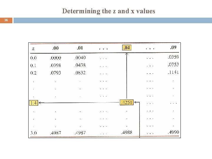
Determining the z and x values 35 We reverse the procedure of finding the area under the normal curve for a specific value of z or x to finding a specific value of z or x for a known area under the normal curve. Ø Example: Find a point z such that the area under the standard normal curve between 0 and z is. 4251 and the value of z is positive

Determining the z and x values 36

Determining the z and x values 37 Example: Find the value of z such that the area under the standard normal curve in the right tail is. 0050.

Determining the z and x values 38 Example: Find the value of z such that the area under the standard normal curve in the left tail is. 050.

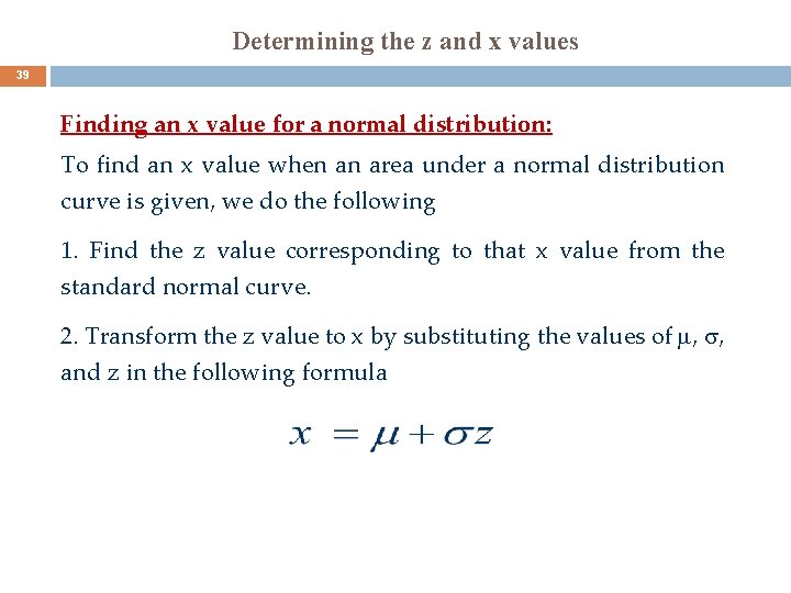
Determining the z and x values 39 Finding an x value for a normal distribution: To find an x value when an area under a normal distribution curve is given, we do the following 1. Find the z value corresponding to that x value from the standard normal curve. 2. Transform the z value to x by substituting the values of , , and z in the following formula

Determining the z and x values 40 Example: Recall the calculators example, it is known that the life of a calculator manufactured by Intal Corporation has a normal distribution with a mean of 54 months and a standard deviation of 8 months. What should the warranty period be to replace a malfunctioning calculator if the company does not want to replace more than 1 % of all the calculators sold

Determining the z and x values 41 Example: Most business schools require that every applicant for admission to a graduate degree program take the GMAT. Suppose the GMAT scores of all students have a normal distribution with a mean of 550 and a standard deviation of 90. Matt Sanger is planning to take this test soon. What should his score be on this test so that only 10% of all the examinees score higher than he does?

Determining the z and x values 42 Example: Find the value of z such that 0. 95 of the area is within ±z standard deviations of the mean