Denotation Firstly we define the denotation of an

算術式のDenotation Firstly, we define the denotation of an arithmetic expression, by structural induction, as a relation between states and numbers: A[[n]] = {(σ, n) | σ∈Σ} A[[X]] = {(σ, σ(X)) | σ∈Σ} A[[a 0 + a 1]] = {(σ, n 0 + n 1) | (σ, n 0) ∈ A[[a 0]] & (σ, n 1) ∈ A[[a 1]] } A[[a 0 – a 1]] = {(σ, n 0 – n 1) | (σ, n 0) ∈ A[[a 0]] & (σ, n 1) ∈ A[[a 1]] } A[[a 0 × a 1]] = {(σ, n 0 × n 1) | (σ, n 0) ∈ A[[a 0]] & (σ, n 1) ∈ A[[a 1]] } An obvious structural induction on arithmetic expressions a shows that each denotation A[[a]] is in fact a function. Notice that the signs “+”, ”－”, ”×” on the lefthand sides represent syntactic signs in IMP whereas the signs on the right represent operations on numbers, so e. g. , for any state σ, A[[3 + 5]]σ = A[[3]]σ+ A[[5]]σ = 3 + 5 = 8, as is to be expected. Note that using λ-notation we can present the definition of the semantics in the following equivalent way: A[[n]] = λσ ∈ Σ. n A[[X]] = λσ ∈ Σ. σ(X) A[[a 0 + a 1]] = λσ ∈ Σ. (A[[a 0]]σ + A[[a 1]]σ) A[[a 0 － a 1]] = λσ ∈ Σ. (A[[a 0]]σ － A[[a 1]]σ) A[[a 0 × a 1]] = λσ ∈ Σ. (A[[a 0]]σ × A[[a 1]]σ)

ブール式のDenotatiion The semantic function for booleans is given in terms of logical operations conjunction ∧T, disjunction ∨T and negation ￢T, on the set of truth values T. The denotation of a boolean expression is defined by structural induction to be a relation between states and truth values. B[[true]] = {(σ, true) | σ∈Σ} B[[false]] = {(σ, false) | σ∈Σ} B[[a 0 = a 1]] = {(σ, true) | σ∈Σ & A[[a 0]]σ = A[[a 1]]σ}∪ {(σ, false) | σ∈Σ & A[[a 0]]σ ≠ A[[a 1]]σ}, B[[a 0 < a 1]] = {(σ, true) | σ∈Σ & A[[a 0]]σ < A[[a 1]]σ}∪ {(σ, false) | σ∈Σ & A[[a 0]]σ < A[[a 1]]σ}, B[[￢b]] = {(σ, ￢Tt) | σ∈Σ & (σ, t) ∈ B[[b]]}, B[[b 0 ∧ b 1]] = {(σ, t 0 ∧T t 1) | σ∈Σ & (σ, t 0) ∈ B[[b 0]] & (σ, t 1) ∈ B[[b 1]]}, B[[b 0 ∨ b 1]] = {(σ, t 0 ∨T t 1) | σ∈Σ & (σ, t 0) ∈ B[[b 0]] & (σ, t 1) ∈ B[[b 1]]}. A simple structural induction shows that each denotation is a function. For example, true if A[[a 0]]σ < A[[a 1]]σ, B[[a 0 < a 1]]σ = false if A[[a 1]]σ < [[a 1]]σ for all σ∈Σ.

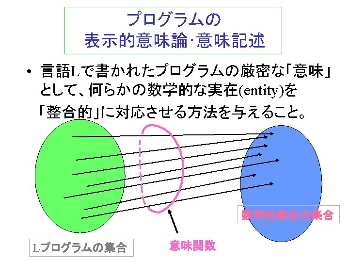
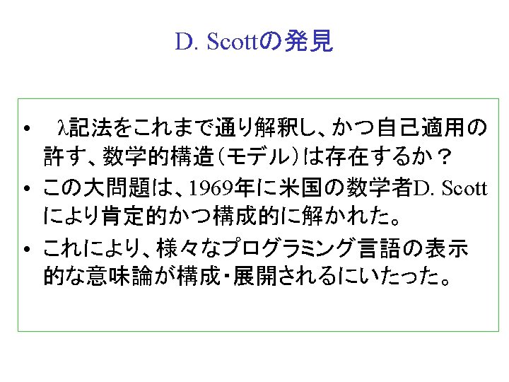
命令文のDenotation The definition of C[[c]] for commands c is more complicated. We will first give denotations as relations between states; afterwards a straightforward structural induction will show that they are, in fact, partial functions. It is fairly obvious that we should take C[[skip]] = {(σ, σ) | σ∈Σ} C[[X : = a]] = {(σ, σ[n/X]) | σ∈Σ & n = A[[a]]σ} 関数/関係の合成、順序に 注意 C[[c 0; c 1]] = C[[c 1]]　C[[C 0]], a composition of relations, the definition of which explains the orderreversal in c 0 and c 1, C[[if b then c 0 else c 1]] = {(σ, σ’) | B[[b]]σ = true & (σ, σ’)∈C[[c 0]]} ∪ {(σ, σ’) | B[[b]]σ = false & (σ, σ’)∈C[[c 1]]}. But there are difficulties when we consider the denotation of a while-loop. Write w ≡ while b do c. We have noted the following equivalence: この等式がポイント 　w ~ if b then c; w else skip so the partial function C[[w]] should equal the partial function C[[if b then c; w else skip]]. Thus we should have: C[[w]] = {(σ, σ’) | B[[b]]σ = true & (σ, σ’) ∈ C[[c; w]]} ∪ {(σ, σ) | B[[b]]σ = false} = {(σ, σ’) | B[[b]]σ = true & (σ, σ’) ∈ C[[w]]○C[[c]]} ∪ {(σ, σ) | B[[b]]σ = false} Writing　　for C [[w]], β for B[[b]] and γ for C[[c]] we require a partial function　　such that = {(σ, σ’) | β(σ) = true & (σ, σ’) ∈　　 ○ γ} ∪　{(σ, σ) | β(σ) = false}. But this involves on both sides of the equation. How can we solve it to find ?

Cont. We clearly require some technique for solving a recursive equation of this form (it is called “recursive” because the value we wish to know on the left recurs on the right). Looked at in another way we can regard Γ, where Γ(　) = {(σ, σ’) | β（σ) = true & (σ, σ’)∈　　γ} ∪ {(σ, σ) | β(σ) = false} = {(σ, σ’) | ∃σ’’. β(σ) = true & (σ, σ’’)∈γ & (σ’’, σ’)∈　}∪ {(σ, σ) | β(σ) = false}, as a function which given　　returns Γ(　). We want a fixed point 　　of Γ in the sense that = Γ( 　). The last chapter provides the clue to finding such a solution in Section 4. 4. It is not hard to check that the function Γ is equal to 　, where 　 is the operator on sets determined by the rule instances 　= {({(σ’’, σ’) / (σ, σ’)) | β(σ) = true & (σ, σ’’)∈γ}∪ {( 　/ (σ, σ)) | β(σ) = false}. As Section 4. 4 shows 　 has a least fixed point = fix(　) where 　is a set　　in this case a set of pairs　　with the property that 　(θ) = θ⇒　　⊆θ. We shall take this least fixed point as the denotation of the while program w. Certainly its denotation should be a fixed point.

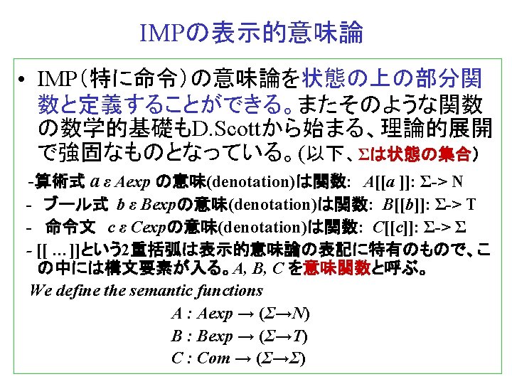
一応のまとめ C[[skip]] = {(σ, σ) | σ∈Σ} C[[X: = a] = {(σ, σ[n/X] | σ∈ Σ& n = A[[a]]σ} C[[c 0; c 1]] = C[[c 1]]　C[[c 0]] C[[if b then c 0 else c 1]] = {(σ, σ’) | Β[[b]]σ = true & (σ, σ’)∈C[[c 0]]}∪ {(σ, σ’) | Β[[b]]σ = false & (σ, σ’)∈C[[c 1]]} C[[while b do c]] = fix(Γ) where Γ(　) = {(σ, σ’) | B[[b]]σ = true & (σ, σ’)∈　　 C[[c]]}∪ {(σ, σ) | Β[[b]]σ = false}. In this way we define a denotation of each command as a relation between states. Notice how the semantic definition is compositional in the sense that the denotation of a command is constructed from the denotations of its immediate subcommands, reflected in the fact that the definition is by structural induction. This property is a hallmark of denotational semantics. Notice it is not true of the operational semantics of IMP because of the rule for while-loops in which the while-loop reappears in the premise of the rule. We have based the definition of the semantic function on while programs by the operational equivalence between while programs and one “unfolding” of them into a conditional. Not surprisingly it is straightforward to check this equivalence holds according to the denotational semantics

課題 Proposition 5. 1 Write ω ≡ while b do c for a command c and boolean expression b. Then C[[ω]] ≡ C[[if b then c; ω else skip]]. Proof: The denotation of ω is a fixed point of Γ, defined above. Hence C[[w]] = Γ(C[[w]]) = {(σ, σ’) | Β[[b]]σ = true & (σ, σ’)∈C[[ω]] C[[c]]}∪ {(σ, σ) | Β[[b]]σ = false} = {(σ, σ’) | Β[[b]]σ = true & (σ, σ’)∈C[[c; ω]]}∪ 　　{(σ, σ’) | Β[[b]]σ = false & (σ, σ’)∈C[[skip]]} =C[[if b then c; ω else skip]]. Exercise 5. 2 Show by structural induction on commands that the denotation C[[c]] is a partial function for all commands c. (The case for while-loops involves proofs by mathematical induction showing that Γn( 　) is a partial function between states for all natural numbers n, and that these form an increasing chain, followed by the observation that the union of such a chain of partial functions is itself a partial function. )

Complete partial orders Definition : A partial order (p. o. ) is a set P on which there is binary relation　　which is: (i) relexive: ∀p∈P. p　 p (ii) transitive: ∀p, q, r∈P. p　 q & q　 r ⇒ p 　r ここが大事 (iii) antisymmetric: ∀p, q∈P. p 　q & q 　p ⇒ p = q. But not all partial orders support the constructions we did on sets. In constructing the least fixed point we formed the union ∪n∈ω An ω-chain A 0⊆A 1⊆・・・An⊆・・・ which started at 　　　the least set. Union on sets, ordered by inclusion, generalises to the notion of least upper bound on partial orders　　we only require them to exist for such increasing chains indexed by ω. Translating these properties to partial orders, we arrive at the definition of a complete partial order. Definition : Let (D, D) be a partial order. An ω-chain of the partial order is an increasing chain d 0　 D d 1 　D・・・ 　D dn 　D・・・ of elements of the partial order. The partial order (D, 　D) is a complete partial order (abbreviated to cpo) if it has　lubs 　of all ω-chains d 0 　D d 1 　D・・・ 　D dn 　D・・・, i. e. any increasing chain {dn | n∈ω} of element in D has a least upper bound 　{dn | n∈ω} in D, often written as 　 n∈ω dn. 　 We say (D, 　D) is a cpo with bottom if it is a cpo which has a least element ⊥D(called “bottom”).

Continuous functions Definition : A function f : D → E be monotonic on between cpos D and E iff for any d and d’ in D, if d d’ then f (d) f (d’) Definition Such a function is continuous iff it is monotonic and for all ω-chains d 0 d 1 　・・・ dn 　・・・ in D, f (dn) = f ( dn). n∈ω An important consequence if this definition is that any continuous function from a cpo with bottom to itself has a least fixed point.

Fixed Point Definition : Let f : D→D be a continuous function on a cpo D. 　　　　　　A fixed point of an element d of D such that f(d) = d. 　　　　　　A prefixed point of f is an element d of D such that f(d) 　d. The following simple, but important, theorem gives an explicit construction fix(f) of the least fixed point of a continuous funciotn f on a cpo D. Theorem 5. 11 (Fixed-Point Theorem) Let f : D→D be a continuous function on a cpo with bottom ⊥. Define fix(f) = 　fn(⊥). n∈ω Then fix(f) is a fixed point of f and the least prefixed point of f i. e. , (i) f(fix(f)) = fix(f) 　　　 (ii) if f(d) 　d then fix(f) 　d. Consequently fix(f) is the least fixed point of f.

The Intuition behind CPO 　We say a little about intuition behind complete partial orders and continuous functions, an intuition which will be discussed further and pinned down more precisely in later chapters. Complete partial orders correspond to types of data, data that can be used as input or output to a computation. Computable functions are modeled as information and the ordering x 　y as meaning x approximates y (or, x is less or the same information as y) so ⊥ is the point of least information. We can recast, into this general framework, the method by which we gave a denotational semantics to IMP. We denoted a command by a partial function from states to states Σ. On the face of it this does not square with the idea that the function computed by a command should be continuous. However partial functions on states can be viewed as continuous total functions. We extend the states by a new element ⊥ to a cpo of results Σ⊥ ordered by ⊥　 σ for all states σ. The cpo Σ⊥ includes the extra element ⊥ representing the undefined state, or more correctly null information about the state, which, as a computation progresses, can grow into the information that a particular final state is determined. It is not hard to see that the partial functions Σ→Σ are in 1 -1 correspondence with the (total) functions Σ→Σ⊥, and that in this case any total function is continuous; the

Continued inclusion order between partial functions corresponds to the “pointwise order” f 　g iff ∀σ∈Σ. f(σ) 　g(σ) between functions Σ→Σ⊥. Because partial functions form a cpo so does the set of functions [Σ→Σ⊥] ordered pointwise. Consequently, our denotational semantics can equivalently be viewed as denoting commands by elements of the cpo of continuous functions [Σ→Σ⊥]. Recall that to give the denotation of a while program we solved a recursive equation by taking the least fixed point of a continuous function on the cpo of partial functions, which now recasts to one on the cpo [Σ→Σ⊥]. For the cpo [Σ→Σ⊥], isomorphic to that of partial functions, more information corresponds to more input/output behavior of a function and no information at all, ⊥ in this cpo, corresponds to the empty partial function which contains no input/output pairs. We can think of the functions themselves as data which can be used or produced by a computation. Notice that the information about such functions comes in discrete units, the input/output pairs. such a discreteness property is shared by a great many of the complete partial orders that arise in modeling computations. As we shall see, that computable functions should be continuous follows from the idea that the appearance of a unit of information in the output of a computable function should only depend on the presence of finitely many units of information in the input. Otherwise a computation yielding that unit of output. We have met this idea before; a set of rule instances determines a continuous operator when the rule instances are finite, in that they have only finite sets of premises.