Demographic PVAs Structured populations Populations in which individuals

Demographic PVAs

Structured populations • Populations in which individuals differ in their contributions to population growth

Population projection matrix model

Population projection matrix model • Divides the population into discrete classes • Tracks the contribution of individuals in each class at one census to all classes in the following census

States • Different variables can describe the “state” of an individual • Size • Age • Stage

Advantages • Provide a more accurate portray of populations in which individuals differ in their contributions to population growth • Help us to make more targeted management decisions

Disadvantages • These models contain more parameters than do simpler models, and hence require both more data and different kinds of data

Estimation of demographic rates • Individuals may differ in any of three general types of demographic processes, the so-called vital rates • Probability of survival • Probability that it will be in a particular state in the next census • The number of offspring it produces between one census and the next

Vital rates • Survival rate • State transition rate (growth rate) • Fertility rate The elements in a projection matrix represent different combinations of these vital rates

The construction of the stochastic projection matrix 1. Conduct a detailed demographic study 2. Determine the best state variable upon which to classify individuals, as well the number and boundaries of classes 3. Use the class-specific vital rate estimates to build a deterministic or stochastic projection matrix model

Conducting a demographic study • Typically follow the states and fates of a set of known individuals over several years • Mark individuals in a way that allows them to be re-identified at subsequent censuses

Ideally • The mark should be permanent but should not alter any of the organism’s vital rates

Determine the state of each individual • Measuring size (weight, height, girth, number of leaves, etc) • Determining age

Sampling • Individuals included in the demographic study should be representative of the population as a whole • Stratified sampling

Census at regular intervals • Because seasonality is ubiquitous, for most species a reasonable choice is to census, and hence project, over one-year intervals

Birth pulse • Reproduction concentrated in a small interval of time each year • It make sense to conduct the census just before the pulse, while the number of “seeds” produced by each parent plant can still be determined

Birth flow • Reproduce continuously throughout the year • Frequent checks of potentially reproductive individuals at time points within an inter-census intervals may be necessary to estimate annual per-capita offspring production or more sophisticated methods may be needed to identify the parents

Special procedures • Experiments • Seed Banks • Juvenile dispersal

Data collection should be repeated • To estimate the variability in the vital rates • It may be necessary to add new marked individuals in other stages to maintain adequate sample sizes

Establishing classes • Because a projection model categorizes individuals into discrete classes but some state variables are often continuous… • The first step in constructing the model is to use the demographic data to decide which state variable to use as the classifying variable, and • if it is continuous, how to break the state variable into a set of discrete classes

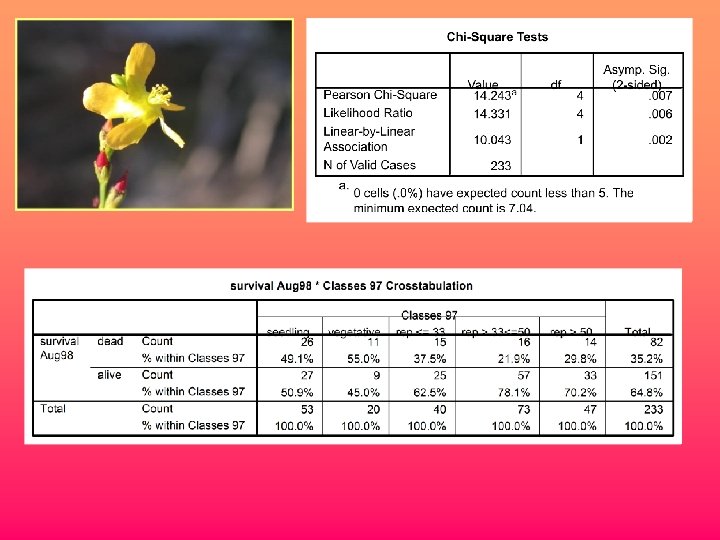
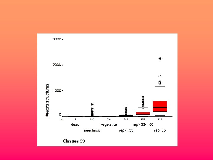
Appropriate Statistical tools for testing associations between vital rates and potential classifying variables Vital rate Classifying variable Survival or reproduction binary Age or size Logistic regression Continuous Stage Discrete Log-linear models Reproduction Discrete but not binary Reproduction or growth Continuous or so Generalized Linear, linear models polynomial or non-linear regression Log-linear ANOVAs models

P (survival) P(survival) (i, t+1)=exp (ßo +ß 1*area (i, t) ) /(1+ exp (ßo +ß 1*area (i, t)))

Growth Area (i, t+1) =Area (i, t)*(1+(exp(ßo +ß 1*ln(Area (i, t) ))))

P (flowering) (i, t+1) = exp (ßo +ß 1*area (i, t) ) /(1+ exp (ßo +ß 1*area (i, t)))

Choosing a state variable • Apart from practicalities and biological rules-of-thumb • An ideal state variable will be highly correlated with all vital rates for a population, allowing accurate prediction of an individual’s reproductive rate, survival, and growth • Accuracy of measurement

Number of flowers and fruits CUBIC r 2 =. 701, n= 642 P <. 0001 y= 2. 8500 -1. 5481 x +. 0577 x 2 +. 0010 x 3

Classifying individuals Hypericum cumulicola

Age 2 -3 different years

Stage different years same cohort

An old friend • AICc = -2(ln. Lmax, s + ln. Lmax, f)+ + (2 psns)/(ns-ps-1) + (2 pfnf)/(nf-pf-1) Growth is omitted for two reasons 1. State transitions are idiosyncratic to the state variable used 2. We can only use AIC to compare models fit to the same data

Setting class boundaries • Two considerations 1. We want the number of classes be large enough that reflect the real differences in vital rates 2. They should reflect the time individuals require to advance from birth to reproduction

Estimating vital rates • Once the number and boundaries of classes have been determined, we can use the demographic data to estimate three types of class-specific vital rates

Survival rates • For stage: • Determine the number of individuals that are still alive at the current census regardless of their state • Dive the number of survivors by the initial number of individuals

Survival rates • For size or age : • Determine the number of individuals that are still alive at the current census regardless of their size class • Dive the number of survivors by the initial number of individuals • But… some estimates may be based on small sample sizes and will be sensitive to chance variation

A solution • Use the entire data set to perform a logistic regression of survival against age or size • Use the fitted regression equation to calculate survival for each class 1. Take the midpoint of each size class for the estimate 2. Use the median 3. Use the actual sizes

State transition rates • We must also estimate the probability that a surviving individual undergoes a transition from its original class to each of the other potential classes

State transition rates

Fertility rates • The average number of offspring that individuals in each class produce during the interval from one census to the next • Stage: imply the arithmetic mean of the number of offspring produced over the year by all individuals in a given stage • Size: use all individuals in the data set

Building the projection matrix

A typical projection matrix A = a 11 a 12 a 13 a 21 a 22 a 23 a 31 a 32 a 33

A matrix classified by age A = 0 F 2 F 3 P 21 0 0 0 P 32 0

A matrix classified by stage A = P 11 F 2 + P 12 F 3 P 21 P 22 0 0 P 32 P 33

Birth pulse, pre breeding fi so Census t fi*so Census t +1

Birth pulse, post breeding sj*fi sj Census t +1

Birth flow √sj*fi *√so Average fertility √sj Census t √so Actual fertility Census t +1

Demographic PVA’s Based on vital rates

Basic types of vital rates • Fertility rates • Survival rates • State transition, or growth rates

The estimation of Vital rates • Accurate estimation of variance and correlation in the demographic rates • We need to know: • The mean value for each vital rate • The variability in each rate • The covariance or correlation between each pair of rates

Limitations of Matrix selection • The assumption that the precise combinations of values that we observed the limited duration of a demographic study will always occur is unlikely to be correct.

A more realistic approach • Use the means, variances, and correlations between vital rates, and then simulate a broader range of possible values

The problem of negative correlations • A hypothetical individual is currently in size class 3 and has mean probability s 3=0. 95 of surviving for one year. • If it survives it will either stay the same size, or grow to be in size class 4 with mean probability g 4, 3=0. 10 a 33=s 3(1 -g 43)=(0. 95)(1 -0. 10) and a 43=s 3 g 43=(0. 95)(0. 10)

The Desert Tortoise

Size classes and definitions of matrix elements for the desert tortoise assuming a prebreeding census Class Yearling Juvenile 1 Juvenile 2 Immature Subadult Adult 1 Adult 2 0 1 2 3 4 5 6 7 0 1 s 2(1 -g 2) s 2 g 2 2 3 4 5 f 5 6 f 6 7 f 7 s 2(1 -g 2) s 2 g 2 s 3(1 -g 3) s 3 g 3 s 4(1 -g 4) s 4 g 4 s 5(1 -g 5) s 5 g 5 s 6(1 -g 6) s 6 g 6 s 7

Estimated vital rates Growth Survival Class 1970 1980 e 1980 l Mean Var 2 . 5 0 0. 5 0. 33 0. 083 . 63 1 . 65 . 76 . 044 3 . 5 0. 18 0. 177 0. 28 0. 036 . 91 1 . 98 . 96 . 002 4 . 47 0. 067 0 0. 18 0. 065 . 98 . 59 . 81 . 79 . 039 5 . 23 0. 26 0 0. 16 0. 020 . 98 . 92 1 . 96 . 0018 6 . 063 0. 032 0. 001 . 99 1 . 68 . 89 . 034 . 78 1 . 86 . 015 7

Pearson Correlations Growth g 2 g 3 g 4 g 5 g 2 1 g 3 . 469 1 g 4 . 382 . 995 1 g 5 -. 597 . 429 . 514 1 g 6 -0. 014 . 877 . 919 . 811 g 6 1

Pearson Correlations Survival s 2 s 3 s 4 s 5 s 6 s 2 1 s 3 . 726 1 s 4 -. 911 -. 945 1 s 5 -. 946 -. 465 . 729 1 s 6 . 487 -. 247 -. 083 -. 743 1 s 7 . 997 . 778 -. 941 -. 918 . 417 s 7 1

Pearson Correlations Survival-Growth s 2 s 3 s 4 s 5 s 6 s 7 g 2 1 -. 704 . 898 . 956 -. 514 -. 994 g 3 . 496 -. 957 . 810 . 189 . 516 -. 563 g 4 -. 41 -. 925 . 75 . 094 . 597 -. 481 g 5 . 571 -. 149 -. 182 -. 806 . 995 . 505 g 6 -0. 017 -. 7 . 428 -. 307 . 865 -. 096

Key distributions for vital rates 0. 5, 0. 001 0. 5, 0. 2 The beta distribution 0. 5, 0. 01

Key distributions for vital rates The beta distribution

Lognormal

Stretched Beta

Matrix selecti on Eleme nt selecti on Vital rate