Demand Forecasting in Supply Chain Learning Objectives n

Demand Forecasting in Supply Chain

Learning Objectives n n Role of forecasting in a supply chain Components of a demand forecast Demand forecasting using historical data Analysing forecast errors 2

Role of forecasting n Demand forecasts form the basis of all planning decisions in a supply chain n Push: produce to anticipated demand levels Pull: set capacity and component availability levels Forecast time horizons n n n Short term (days, weeks): shift scheduling Medium Term (weeks, months): workforce planning, materials purchasing, promotions Long term (months, years): capacity expansion, capital/financial budget 3

Characteristics of Forecasts n Forecasts are always wrong! n n n Expected value Error/variability from the expected value Long-term forecasts are usually less accurate than short-term forecasts Aggregate forecasts are usually more accurate than disaggregate forecasts Mature products with stable demand are easier to forecast than seasonal goods or “fashion” items with short product-life 4

Influences on Customer Demand “Predictions are usually difficult, especially about the future” – Yogi Berra n Historical patterns n n n Externalities n n n Weather State of the economy Internal factors n n n Past demand -> future demand Seasonality? Trend? Planned promotional/discount campaigns Display position and advertising efforts Competitors’ actions 5

Components of Observed Demand Observed demand (O) = Systematic component (S) + Random component (R) n Forecasting should focus on identifying the systematic component n Systematic component = Expected value of demand Time series model: n (Basic) demand level n Trend, rate of growth/decline in demand period n Seasonality, (predictable) seasonal fluctuations n 6

Components of Observed Demand n A Random Component measures the fluctuations in demand from the expected value of demand by analyzing the uncontrollable factors and estimating the forecast error which is a very important input to supply chain managers in forecasting the demand. 7

Forecasting Methods n n Types of Forecasting Methods depend on the time frame, demand behavior and causes of the behavior. Time Frame Indicates how far into the future is the forecast which can be short range, medium range and long range based on the time frame. Short- to mid-range forecast typically encompasses the immediate future, which may be from daily up to two years time period. Long-range forecast will encompass a period of time which is longer than two years. 8

Forecasting Methods n n Demand Behavior can be categorized as a trend, random variations, cyclical and seasonal pattern. Trend behavior is a defined as a gradual, long-term up or down movement of demand. Random variations are defined as the movement in demand that do not follow a specific pattern. Cyclical behavior is defined as an up-and-down repetitive movement in demand. Seasonal pattern of behavior is defined as an upand-down repetitive movement of demand occurring periodically. 9

Forecasting Methods n n Qualitative forecast methods are Subjective in nature. They use judgement, intuition, expertise opinion to produce quantitative estimate of the future demand. When historical data is not available this method is used to estimate the future demand. Experts who have good market intelligence make such decisions. Quantitative forecast methods are Objective in nature and are based on numerical data and application of mathematical formulas. They are classified as Time Series analysis, Casual analysis and Simulation analysis. 10

Forecasting Methods n Time Series n n Causal n n n Assume past history is good indicator of future demand Best for stable environments Easy to implement Assume other (measurable) factors that is correlated with demand Models (e. g. regression) identify factors and quantifies the strength of the correlations Simulation n Assumes some underlying principles of customer behaviour and develop possible scenarios in the future to predict demand 11

Forecasting Methods n n Time Series Analysis: When historical data are available, we use time series analysis to estimate the demand for a short term period of six months, which will be accurate. Time series is a statistical technique that uses historical demand data to predict future demand. Time Series assume that the environment and factors of consideration what has occurred in the past will continue to remain the same in the future too. It relates the forecast to only one factor – time. This method is simple and easy to forecast the demand. 12

Forecasting Methods n n Linear trend line method, moving average method, exponential smoothing are few time series analysis methods of forecasting. Linear trend is a technique which fits a linear trend line using a mathematical equation involving the Independent variable, Dependant variable and constants. 13

Forecasting Methods n n A moving average is an indicator that shows the average value over a period of time. Simple moving averages apply equal weight to the data over a period of time. Exponential smoothing is a moving average method which applies more weight to recent data over the time period to forecast the demand. 14

Forecasting Methods n n Casual Analysis: A casual method of forecasting uses the relationship between the various demand factors of the supply chain and their relationship to estimate the demand for the future. This method would be a good forecasting method for a medium to long term period. This method is prone to substantial forecasting error. Correlation and Regression methods are used to estimate the future demand under this method. 15

Forecasting Methods n n Correlation is a measure of the strength of the relationship between independent and dependent variables. Regression method is an attempt to develop a mathematical relationship between demand factors that cause its behavior. Linear regression is a mathematical technique that relates a dependent variable to an independent variable in the form of a linear equation. 16

Forecasting Methods n Simulation Analysis: n This method imitates the situation and predicts the demand for the product. Algorithms are formulated to estimate the demand. 17

Forecasting Error n n n When the future forecast is not perfectly estimated based on the past, the future forecast will have an error to some degree. The error in the forecast is referred to as forecast error which is the difference between the forecast and the actual. Mathematically it is given by Et = Ft - Dt, Where Et is the forecast error in period t, Ft is the forecasted demand in period t and Dt, is the actual demand in period t. 18

Forecasting Error n n The forecast error is a risk in demand planning. Longer lead times, seasonality of the products, shorter life cycle of the product, catering to a niche market, etc, . are the factors leading to the forecast error creating the risk in demand planning. To manage the risk two strategies can be adopted by the supply chain manager, namely increased responsiveness of the supply chain and pooling of demand. 19

Basic Approach to Demand Forecasting n Understand the objective of forecasting n n Integrate demand planning and forecasting n n n Levels of aggregation Determine the appropriate forecasting technique n n Growth Trend? Seasonality? Substitutes and complementary products? Understand identify customer segments n n Co-ordination between marketing, production and suppliers Identify major factors that influence the demand forecast n n Forecast horizon; affected by suppliers’ lead times Geographical location, product life-cycle, etc. Establish performance and error measures forecasts n Assess cost impacts; consider investments in improving forecasts accuracies No forecast is perfect; system must be flexible and have contingency plans to handle forecast errors 20

Common Time Series Patterns n n Constant (stationary) Increasing/decreasing linear trend Seasonal variations Non-linear (e. g. exponential) trend 21

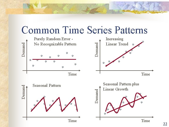
Purely Random Error No Recognizable Pattern Demand Common Time Series Patterns Increasing Linear Trend Time Seasonal Pattern Demand Time Seasonal Pattern plus Linear Growth Time 22

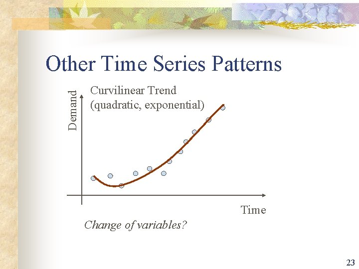
Demand Other Time Series Patterns Curvilinear Trend (quadratic, exponential) Time Change of variables? 23

Static Forecasting n Methods: n n Simple averaging Linear regression 24

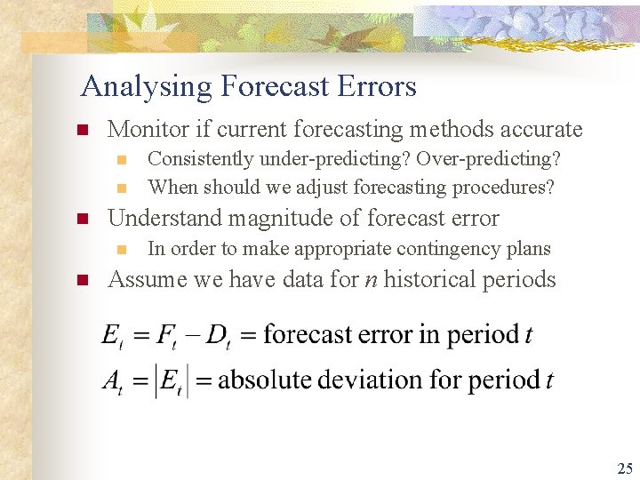
Analysing Forecast Errors n Monitor if current forecasting methods accurate n n n Understand magnitude of forecast error n n Consistently under-predicting? Over-predicting? When should we adjust forecasting procedures? In order to make appropriate contingency plans Assume we have data for n historical periods 25

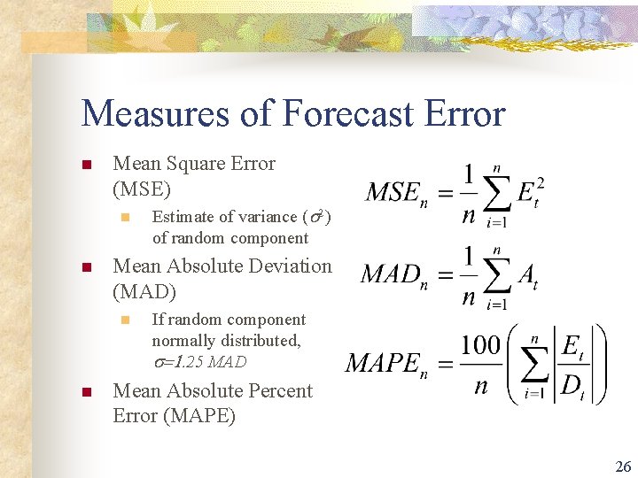
Measures of Forecast Error n Mean Square Error (MSE) n n Mean Absolute Deviation (MAD) n n Estimate of variance (s 2) of random component If random component normally distributed, s=1. 25 MAD Mean Absolute Percent Error (MAPE) 26

Summary so far n n n Importance of forecasting in a supply chain Forecasting models and methods Exponential smoothing n n n Stationary model Trend Seasonality Measures of forecast errors Regression models SEG 4610 Forecasting 27

Regression Analysis n n Statistical technique to determine the degree of association between set of variables and demand. Given values of the predictor (independent) variables, the regression equation provides a forecast of demand. SEG 4610 Forecasting 28

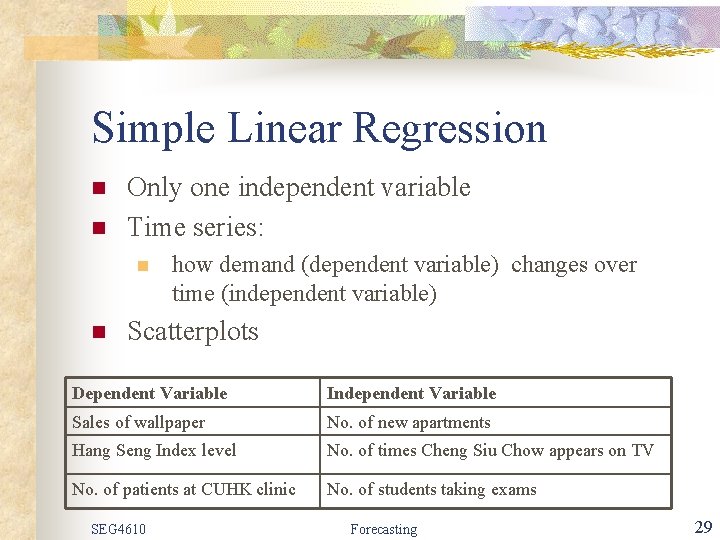
Simple Linear Regression n n Only one independent variable Time series: n n how demand (dependent variable) changes over time (independent variable) Scatterplots Dependent Variable Independent Variable Sales of wallpaper No. of new apartments Hang Seng Index level No. of times Cheng Siu Chow appears on TV No. of patients at CUHK clinic No. of students taking exams SEG 4610 Forecasting 29

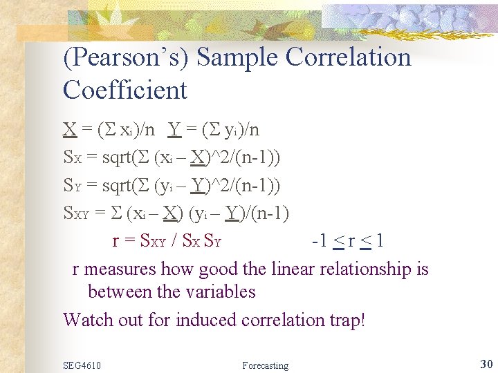
(Pearson’s) Sample Correlation Coefficient X = (S xi)/n Y = (S yi)/n SX = sqrt(S (xi – X)^2/(n-1)) SY = sqrt(S (yi – Y)^2/(n-1)) SXY = S (xi – X) (yi – Y)/(n-1) r = SXY / SX SY -1 < r < 1 r measures how good the linear relationship is between the variables Watch out for induced correlation trap! SEG 4610 Forecasting 30

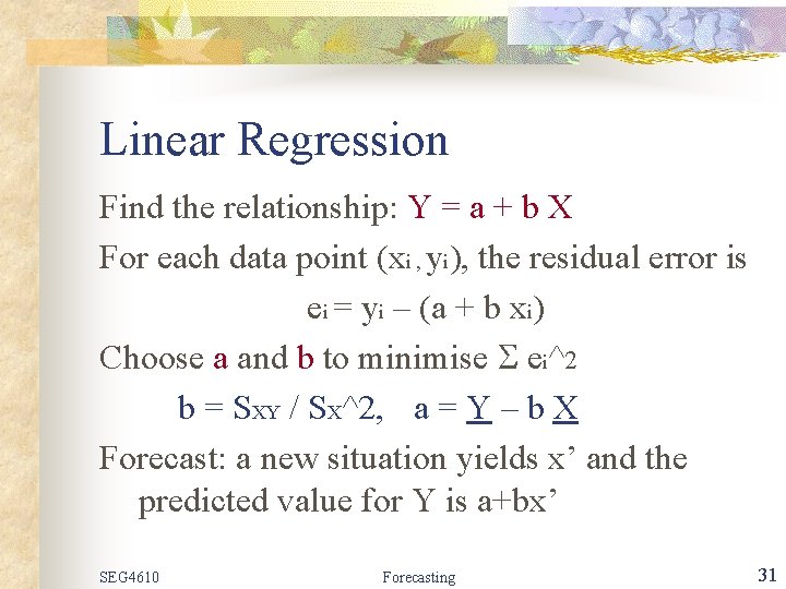
Linear Regression Find the relationship: Y = a + b X For each data point (xi , yi), the residual error is ei = yi – (a + b xi) Choose a and b to minimise S ei^2 b = SXY / SX^2, a = Y – b X Forecast: a new situation yields x’ and the predicted value for Y is a+bx’ SEG 4610 Forecasting 31

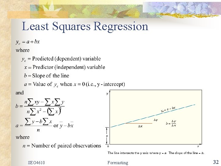
Least Squares Regression SEG 4610 Forecasting 32

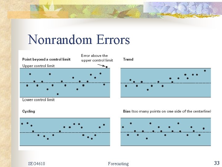
Nonrandom Errors SEG 4610 Forecasting 33

Special Forecasting Difficulties for Supply Chains n New products and service introductions n n n Lumpy derived demand n n No past history Use qualitative methods until sufficient data collected Examine correlation with similar products Use a large exponential smoothing constant Large but infrequent orders Random variations “swamps” trend and seasonality Identify reason for lumpiness and modify forecasts Spatial variations in demand n Separate forecast vs. allocation of total forecasts 34