Demand Forecasting Demand Estimation Techniques Qualitative Consumer Surveys

Demand Forecasting

Demand Estimation Techniques Qualitative - Consumer Surveys - Market Experiments - Consumer Clinics - Virtual Shopping Quantitative - Statistical Techniques Regression Every decision maker has to plan for the future and a reliable prediction helps reduce uncertainty of the environment in which managerial decisions are made.

Consumer Surveys: • It involves gathering of information about consumer behavior from a sample of consumers which is analyzed and then further projected onto the population. • Surveys are conducted to assess consumers perception of various aspects, such as new variations in products, variations in prices of the product and related products, new variations in services provided etc. • The drawback of this method is that the consumer has to respond to hypothetical situations.

Market experiments: • Seller of a product introduces variations and tries it out in a representative market. • The seller gathers information on the behavior of the consumers in this representative market. • This is a high cost technique. • Advantage of market experiments are that they can be conducted on a large scale to ensure validity of results and consumers are not aware that they are a part of experiments.

Consumer Clinics: • Consumers are asked to act in a simulated situation, wherein they are given a certain sum of money and made to indulge in buying and their behavior is observed. • These are laboratory experiments. Participants have an incentive to purchase the commodity as they are usually allowed to keep the goods purchased.

Virtual Shopping – A representative sample of consumers shop in a virtual store simulated on the computer screen. – By doing so, this method eliminates the high cost in terms of time and money involved in consumer clinics. – Sample customers are asked to take a series of trips through the simulated virtual store. – Prices, packaging, displays and promotions are changed in subsequent trips and consumer reaction recorded.

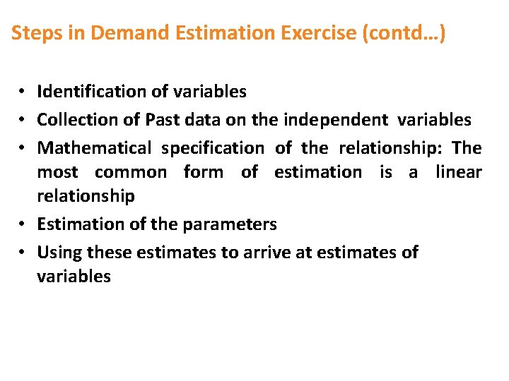
Steps in Demand Estimation Exercise Drawback of relying on direct methods such as surveys is that the data can be unrealistic. A more effective method is to rely on historical data. • Identification of variables: We are required to identify the variable which affect the demand function for a particular product. • Specification of the model: More than one specific form is required to arrive at the best possible form that captures the relationship. It could be linear or exponential. However, the most common is linear.

Steps in Demand Estimation Exercise • Collecting historical data: Next step involves collecting past data on each of the variables. The demand for the subject matter of the study is the dependent variable. The number of data items required is governed by the optimal sample size though it is known that the larger the better. • A set of techniques which uses historical data and enables us to estimate the demand relationships, is covered under the subject matter of econometrics.

Steps in Demand Estimation Exercise (contd…) • Identification of variables • Collection of Past data on the independent variables • Mathematical specification of the relationship: The most common form of estimation is a linear relationship • Estimation of the parameters • Using these estimates to arrive at estimates of variables

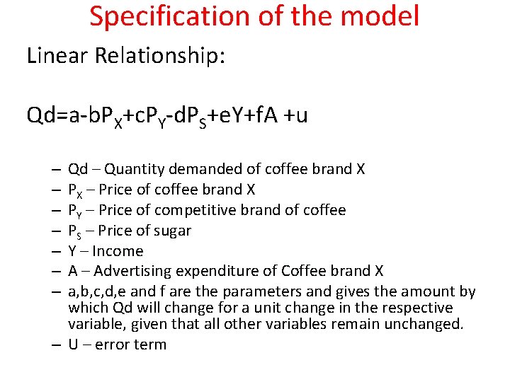
Specification of the model Linear Relationship: Qd=a-b. PX+c. PY-d. PS+e. Y+f. A +u Qd – Quantity demanded of coffee brand X PX – Price of coffee brand X PY – Price of competitive brand of coffee PS – Price of sugar Y – Income A – Advertising expenditure of Coffee brand X a, b, c, d, e and f are the parameters and gives the amount by which Qd will change for a unit change in the respective variable, given that all other variables remain unchanged. – U – error term – – – –

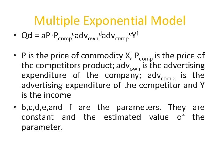
Multiple Exponential Model • Qd = a. Pb. Pcompcadvowndadvcompe. Yf • P is the price of commodity X, Pcomp is the price of the competitors product; advown is the advertising expenditure of the company; advcomp is the advertising expenditure of the competitor and Y is the income • b, c, d, e, and f are the parameters. They are constant and the estimated value of the parameter.

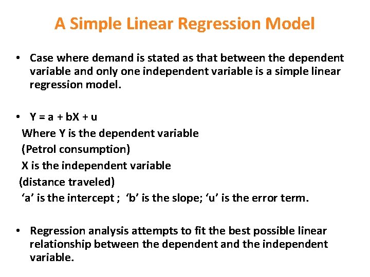
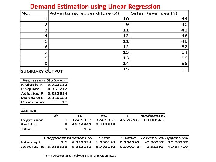
A Simple Linear Regression Model • Case where demand is stated as that between the dependent variable and only one independent variable is a simple linear regression model. • Y = a + b. X + u Where Y is the dependent variable (Petrol consumption) X is the independent variable (distance traveled) ‘a’ is the intercept ; ‘b’ is the slope; ‘u’ is the error term. • Regression analysis attempts to fit the best possible linear relationship between the dependent and the independent variable.

Demand Estimation using Linear Regression

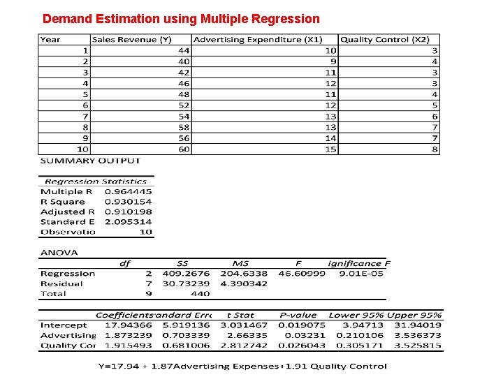
Demand Estimation using Multiple Regression

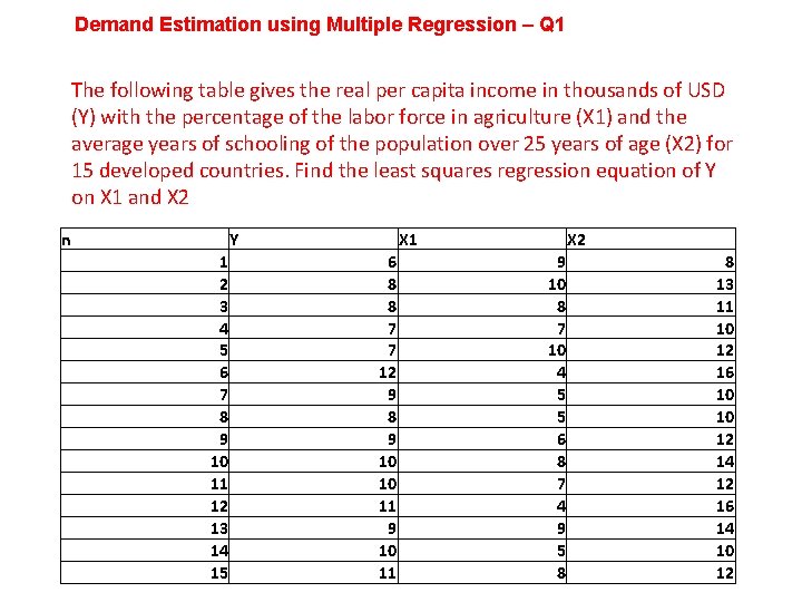
Demand Estimation using Multiple Regression – Q 1 The following table gives the real per capita income in thousands of USD (Y) with the percentage of the labor force in agriculture (X 1) and the average years of schooling of the population over 25 years of age (X 2) for 15 developed countries. Find the least squares regression equation of Y on X 1 and X 2 n Y 1 2 3 4 5 6 7 8 9 10 11 12 13 14 15 X 1 6 8 8 7 7 12 9 8 9 10 10 11 9 10 11 X 2 9 10 8 7 10 4 5 5 6 8 7 4 9 5 8 8 13 11 10 12 16 10 10 12 14 12 16 14 10 12

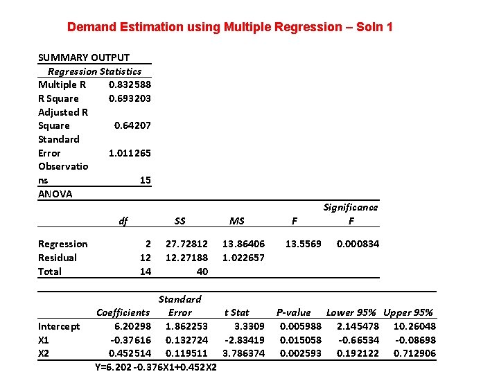
Demand Estimation using Multiple Regression – Soln 1 SUMMARY OUTPUT Regression Statistics Multiple R 0. 832588 R Square 0. 693203 Adjusted R Square 0. 64207 Standard Error 1. 011265 Observatio ns 15 ANOVA df Regression Residual Total Intercept X 1 X 2 SS 2 12 14 27. 72812 12. 27188 40 MS 13. 86406 1. 022657 Standard Coefficients Error t Stat 6. 20298 1. 862253 3. 3309 -0. 37616 0. 132724 -2. 83419 0. 452514 0. 119511 3. 786374 Y=6. 202 -0. 376 X 1+0. 452 X 2 F 13. 5569 Significance F 0. 000834 P-value Lower 95% Upper 95% 0. 005988 2. 145478 10. 26048 0. 015058 -0. 66534 -0. 08698 0. 002593 0. 192122 0. 712906

Regression …. • There again two types of data • i) Time Series ii) Cross section • Sales of cars over the past five years is an example of time series data. • Sales of cars in metros of India during 2007 -08 is an example of cross-sectional data.

Regression …. • Based on either time series or cross sectional data, the estimate procedure sets out to estimate the parameters of the model, ie, the slope b and intercept a respectively. • Estimating the parameters of the model: Method of ordinary least squares (OLS), wherein the method draws a line through the scatter of data in such a way that sum of the squared deviations of each of the points from the line is minimized.

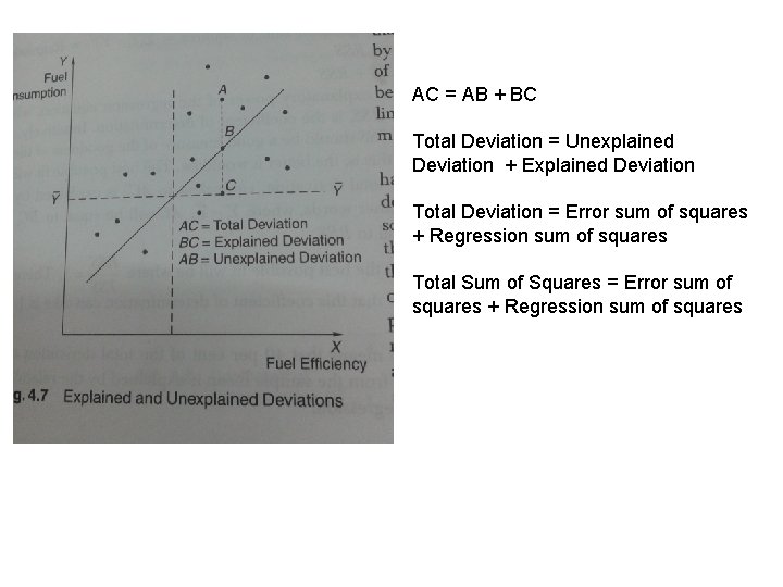
Coefficient of Determination • Coefficient of determination is defined as the proportion of the total variation or dispersion in the dependent variable that is explained by the variation in the independent or explanatory variable. In our eg: variation in petrol consumption due to distance traveled. • Coefficient of determination determines how well a regression line fits the scatter of points:

AC = AB + BC Total Deviation = Unexplained Deviation + Explained Deviation Total Deviation = Error sum of squares + Regression sum of squares Total Sum of Squares = Error sum of squares + Regression sum of squares

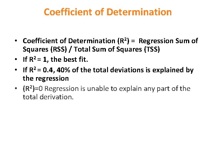
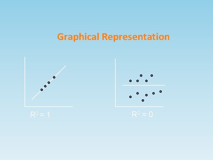
Coefficient of Determination • Coefficient of Determination (R 2) = Regression Sum of Squares (RSS) / Total Sum of Squares (TSS) • If R 2 = 1, the best fit. • If R 2 = 0. 4, 40% of the total deviations is explained by the regression • (R 2)=0 Regression is unable to explain any part of the total derivation.

Graphical Representation R 2 = 1 R 2 = 0

Coefficient of Determination • There is no established objective level for a good established R 2. • Ratio of RSS to TSS is a good measure of goodness of fit and the higher this is, the better it would be. • All other things remaining same, a time series data gives a regression with a higher R 2 than cross sectional data.

Problems in using Regression • Multicollinearity – where there is dependency amongst independent variables. This refers to the situation in which two or more explanatory variables in the regression analysis are highly correlated.

Problems in using Regression • Auto correlation occurs when the dependent variable is related to an independent variable in a specific pattern. Autocorrelation increases chances of null hypothesis being rejected when it may not be the case. Variable might be considered statistically significant, when it may not be so.

Forecasting of demand • Involves projecting the values of the present to a future point in time. It is a difficult task. Statisticians have worked out some models for the purpose. • Aim of economic forecasting is to reduce the risk or uncertainty that the firm faces in it’s short term operational decision making and in planning for it’s long term growth. • Distinction between estimation and forecast: • A forecast is a projection of the relevant variable, not concerned about underlying factors and their behavior.

Forecasting… • Demand estimation involves primarily understanding the underlying factors or variables and their behavior and effects on the relevant variable. It attempts to understand why and to what extent is the estimate influenced by a variable or a group of variables. • Demand forecast does not go into such relationships, it only attempts to project future demands.

Demand forecasting A demand forecast has to be knit into the rest of the system, and should not be taken in isolation like: • Capacity installation or expansion • Hiring of labor and other related activities • Changes into political and economic environment • It should be based on thorough knowledge and data relating to the past. • Even with these considerations forecast may be far different from real situation All rights reserved

Economic Forecasting • Forecasting involves projecting the values of a variable to a future point in time from what it is at present and what it was in the past, not concerned about the underlying factors and relationships between this variable and others. • Forecasts can be short run or long run. It could be daily, weekly, monthly, quarterly, annual or five / ten or twenty years.

Forecasting Techniques • • • Opinion polls and market research Expert opinion Surveys Trend Analysis Projection Techniques Econometric Models

Forecasting Techniques (contd. ) • Opinion Polls – Opinion polls are conducted on various issues. The issues could be political, economic, product related, market related etc. • Such polls are useful in detecting future trends and changes in trends which quantitative techniques might not be able to capture. • Market research uses the technique extensively to gather information on consumers behavior in the marketplace with respect to a specific product or product category. • Expert Opinion involves seeking the opinion of experts on a subject matter. • Forecasts are generated by a group of expert executives.

Forecasting Techniques (contd. ) • The Delphi method is a systematic, interactive forecasting method which relies on a panel of independent experts. • The carefully selected experts answer questionnaires in two or more rounds. After each round, a facilitator provides an anonymous summary of the experts’ forecasts from the previous round as well as the reasons they provided for their judgments. • Thus, participants are encouraged to revise their earlier answers in light of the replies of other members of the group.

• It is believed that during this process the range of the answers will decrease and the group will converge towards the "correct" answer. • Finally, the process is stopped after a pre-defined stop criterion (e. g. number of rounds, achievement of consensus, stability of results) and the mean or median scores of the final rounds determine the results

Forecasting Techniques (contd. ) • Surveys • Econometric Models: These give an estimate of the dependent variable (which could also be a forecast), if the independent variables used as data are forecasts. Eg: The demand of automobiles which is a function of disposable income, family size, interest rates and index of industrial production could be used to forecast the demand for automobiles.

Forecasting Techniques (contd…. ) • Trend analysis relies on historical data to predict the future. It is the use of historical data to discern a long run trend. – The simplest form of forecasting using trend analysis is the projection into the future of the current value of an economic variable. – Eg: One might forecast that next year sales would be a function of sales in the existing year or alternately next year sales would be a function of this year’s sales and the change in sales between this year and last year. Or a forecaster might predict next year sales based on sketching a line that appears to best fit the historical data. – Models that use only trend analysis might not be that useful as against those which also take into consideration seasonal and cyclical factors.

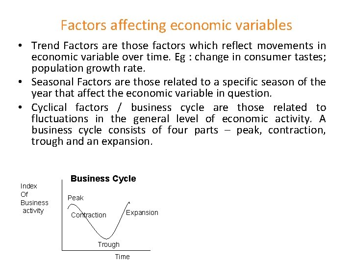
Factors affecting economic variables • Trend Factors are those factors which reflect movements in economic variable over time. Eg : change in consumer tastes; population growth rate. • Seasonal Factors are those related to a specific season of the year that affect the economic variable in question. • Cyclical factors / business cycle are those related to fluctuations in the general level of economic activity. A business cycle consists of four parts – peak, contraction, trough and an expansion. Index Of Business activity Business Cycle Peak Expansion Contraction Trough Time

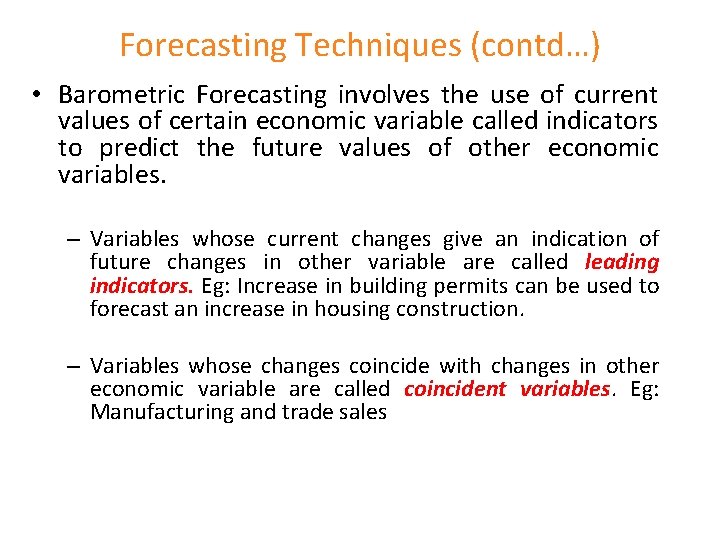
Forecasting Techniques (contd…) • Barometric Forecasting involves the use of current values of certain economic variable called indicators to predict the future values of other economic variables. – Variables whose current changes give an indication of future changes in other variable are called leading indicators. Eg: Increase in building permits can be used to forecast an increase in housing construction. – Variables whose changes coincide with changes in other economic variable are called coincident variables. Eg: Manufacturing and trade sales

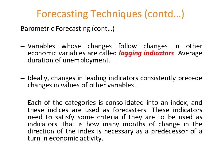
Forecasting Techniques (contd…) Barometric Forecasting (cont…) – Variables whose changes follow changes in other economic variables are called lagging indicators. Average duration of unemployment. – Ideally, changes in leading indicators consistently precede changes in values of other variables. – Each of the categories is consolidated into an index, and these indices are used as forecasters. These indicators need to satisfy some criteria if they are to be used as indicators, that is how many months of change in the direction of the index is necessary as a predecessor of a turn in economic activity.

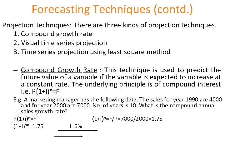
Forecasting Techniques (contd. ) Projection Techniques: There are three kinds of projection techniques. 1. Compound growth rate 2. Visual time series projection 3. Time series projection using least square method – Compound Growth Rate : This technique is used to predict the future value of a variable if the variable is expected to increase at a constant rate. The underlying principle is of compound interest i. e. P(1+i)n=F E. g: A marketing manager has the following data. The sales for year 1990 are 4000 and for year 2000 are 7000. No. of years is 10. What is the compound annual sales growth rate? P(1+i)n=F/P=7000/2000=1. 75 (1+i)10=1. 75 i=6%

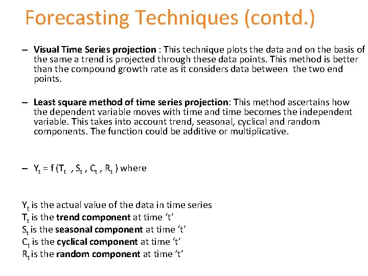
Forecasting Techniques (contd. ) – Visual Time Series projection : This technique plots the data and on the basis of the same a trend is projected through these data points. This method is better than the compound growth rate as it considers data between the two end points. – Least square method of time series projection: This method ascertains how the dependent variable moves with time and time becomes the independent variable. This takes into account trend, seasonal, cyclical and random components. The function could be additive or multiplicative. – Yt = f (Tt , St , Ct , Rt ) where Yt is the actual value of the data in time series Tt is the trend component at time ‘t’ St is the seasonal component at time ‘t’ Ct is the cyclical component at time ‘t’ Rt is the random component at time ‘t’