DEMAND ANALYSIS OVERVIEW of Chapter 3 Demand Relationships

DEMAND ANALYSIS OVERVIEW of Chapter 3 • • • Demand Relationships Demand Elasticities Income Elasticities Cross Elasticities of Demand Appendix 3 A: Indifference Curves 2002 South-Western Publishing Slide 1

Health Care & Cigarettes • Raising cigarette taxes reduces smoking » In Canada, $4 for a pack of cigarettes reduced smoking 38% in a decade • But cigarette taxes also helps fund health care initiatives » The issue then, should we find a tax rate that maximizes tax revenues? » Or a tax rate that reduces smoking? Slide 2

Demand Analysis • An important contributor to firm risk arises from sudden shifts in demand for the product or service. • Demand analysis serves two managerial objectives: (1) it provides the insights necessary for effective management of demand, and (2) it aids in forecasting sales and revenues. Slide 3

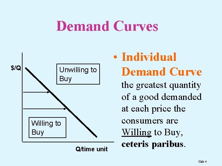
Demand Curves $/Q Unwilling to Buy Willing to Buy Q/time unit • Individual Demand Curve the greatest quantity of a good demanded at each price the consumers are Willing to Buy, ceteris paribus. Slide 4

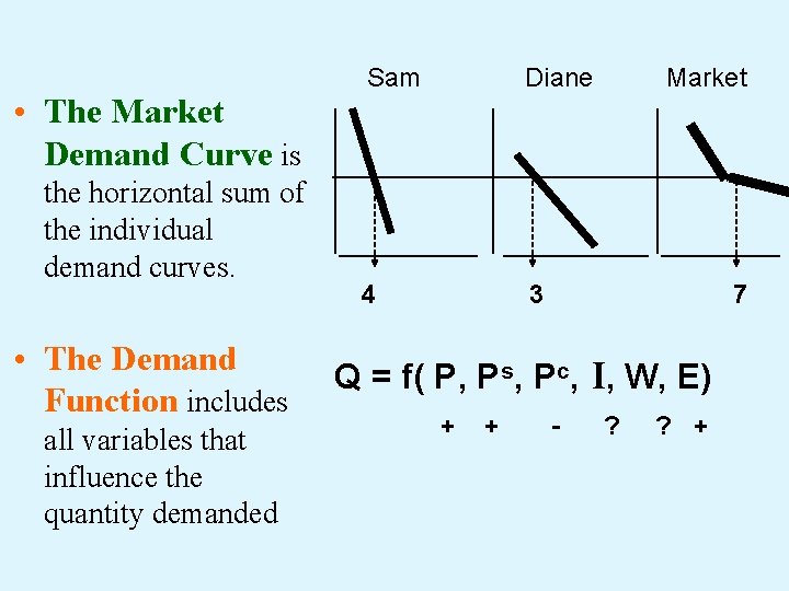
• The Market Demand Curve is the horizontal sum of the individual demand curves. • The Demand Function includes all variables that influence the quantity demanded Sam Diane 4 3 Market 7 Q = f( P, Ps, Pc, I, W, E) + + - ? ? +

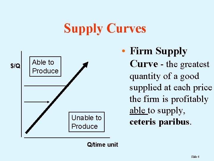
Supply Curves $/Q • Firm Supply Curve - the greatest Able to Produce Unable to Produce quantity of a good supplied at each price the firm is profitably able to supply, ceteris paribus. Q/time unit Slide 6

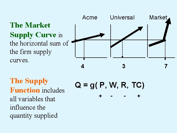
Acme Universal Market The Market Supply Curve is the horizontal sum of the firm supply curves. The Supply Function includes all variables that influence the quantity supplied 4 3 7 Q = g( P, W, R, TC) + - - +

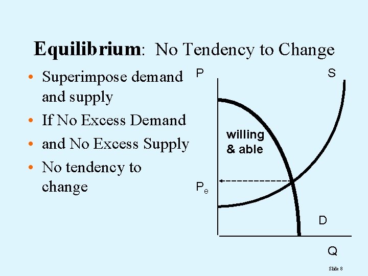
Equilibrium: No Tendency to Change • Superimpose demand supply • If No Excess Demand • and No Excess Supply • No tendency to change P S willing & able Pe D Q Slide 8

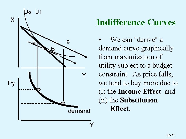
Downward Slope • Reasons that price and quantity are negatively related include: » income effect--as the price of a good declines, the consumer can purchase more of all goods since his or her real income increased. » substitution effect--as the price declines, the good becomes relatively cheaper. A rational consumer maximizes satisfaction by reorganizing consumption until the marginal utility in each good per dollar is equal: • Optimality Condition is MUA/PA = MUB/PB = MUC/PC =. . . If MU per dollar in A and B differ, the consumer can improve utility by purchasing more of the one with higher MU per dollar. Slide 9

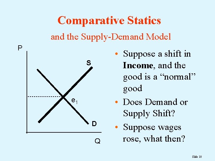
Comparative Statics and the Supply-Demand Model P S e 1 D Q • Suppose a shift in Income, and the good is a “normal” good • Does Demand or Supply Shift? • Suppose wages rose, what then? Slide 10

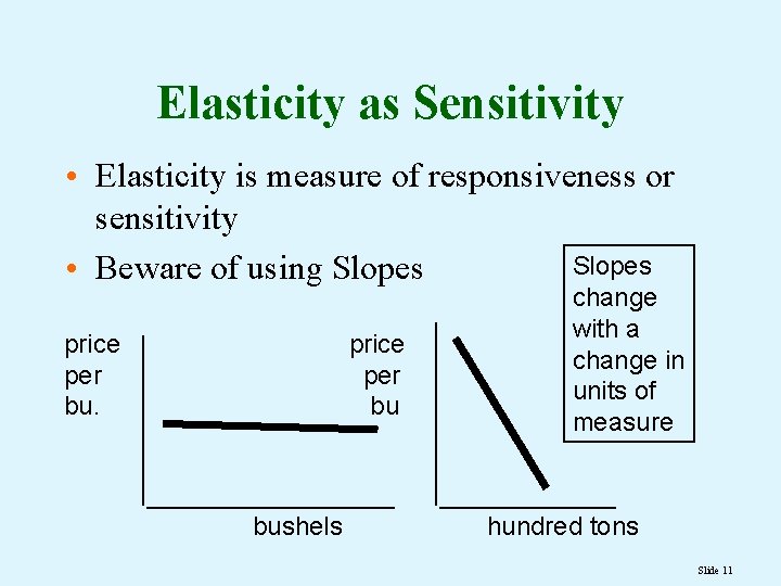
Elasticity as Sensitivity • Elasticity is measure of responsiveness or sensitivity Slopes • Beware of using Slopes price per bu bushels change with a change in units of measure hundred tons Slide 11

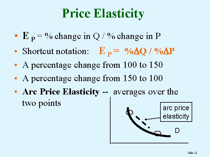
Price Elasticity • E P = % change in Q / % change in P • Shortcut notation: E P = % Q / % P • A percentage change from 100 to 150 • A percentage change from 150 to 100 • Arc Price Elasticity -- averages over the two points arc price elasticity D Slide 12

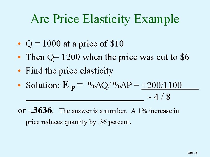
Arc Price Elasticity Example • Q = 1000 at a price of $10 • Then Q= 1200 when the price was cut to $6 • Find the price elasticity • Solution: E P = % Q/ % P = +200/1100 -4/8 or -. 3636. The answer is a number. A 1% increase in price reduces quantity by. 36 percent. Slide 13

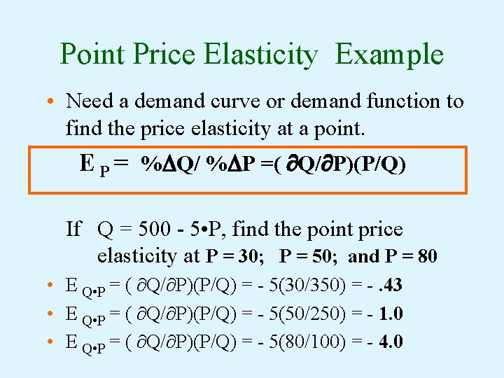
Point Price Elasticity Example • Need a demand curve or demand function to find the price elasticity at a point. E P = % Q/ % P =( Q/ P)(P/Q) If Q = 500 - 5 • P, find the point price elasticity at P = 30; P = 50; and P = 80 • E Q • P = ( Q/ P)(P/Q) = - 5(30/350) = -. 43 • E Q • P = ( Q/ P)(P/Q) = - 5(50/250) = - 1. 0 • E Q • P = ( Q/ P)(P/Q) = - 5(80/100) = - 4. 0

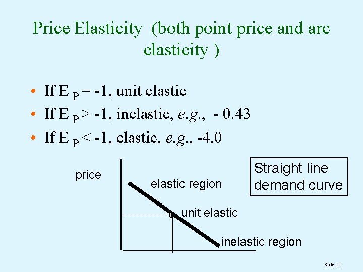
Price Elasticity (both point price and arc elasticity ) • If E P = -1, unit elastic • If E P > -1, inelastic, e. g. , - 0. 43 • If E P < -1, elastic, e. g. , -4. 0 price elastic region Straight line demand curve unit elastic inelastic region Slide 15

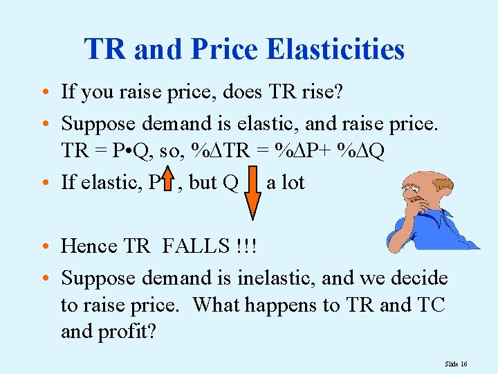
TR and Price Elasticities • If you raise price, does TR rise? • Suppose demand is elastic, and raise price. TR = P • Q, so, % TR = % P+ % Q • If elastic, P , but Q a lot • Hence TR FALLS !!! • Suppose demand is inelastic, and we decide to raise price. What happens to TR and TC and profit? Slide 16

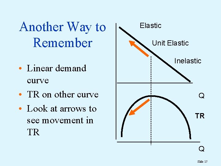
Another Way to Remember • Linear demand curve • TR on other curve • Look at arrows to see movement in TR Elastic Unit Elastic Inelastic Q TR Q Slide 17

1979 Deregulation of Airfares • • Prices declined Passengers increased Total Revenue Increased What does this imply about the price elasticity of air travel ? Slide 18

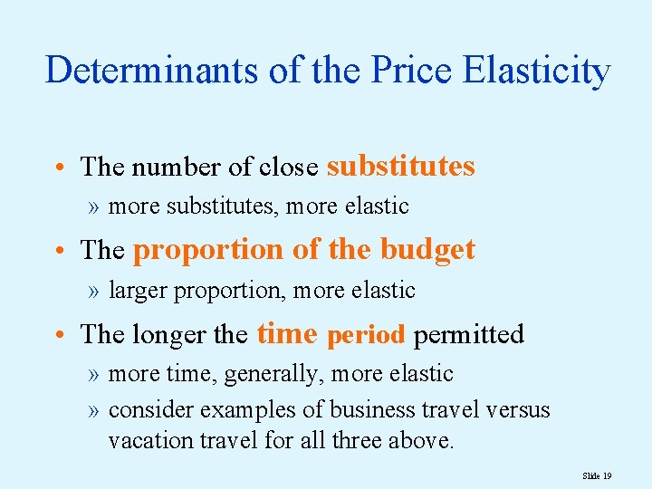
Determinants of the Price Elasticity • The number of close substitutes » more substitutes, more elastic • The proportion of the budget » larger proportion, more elastic • The longer the time period permitted » more time, generally, more elastic » consider examples of business travel versus vacation travel for all three above. Slide 19

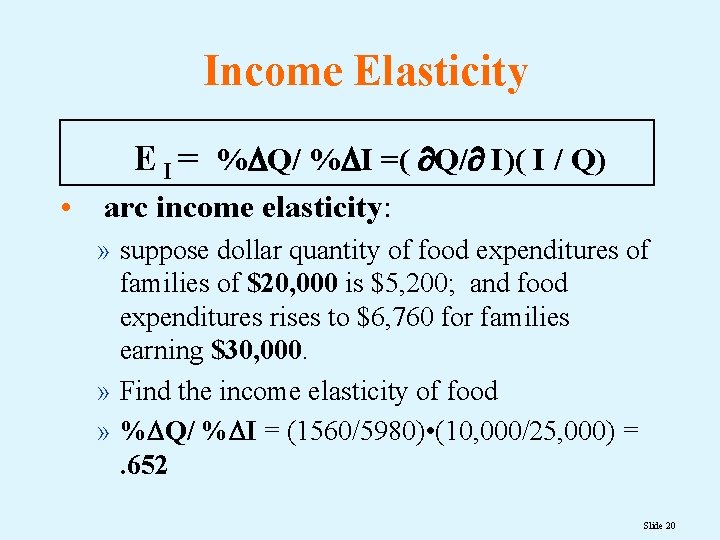
Income Elasticity E I = % Q/ % I =( Q/ I)( I / Q) • arc income elasticity: » suppose dollar quantity of food expenditures of families of $20, 000 is $5, 200; and food expenditures rises to $6, 760 for families earning $30, 000. » Find the income elasticity of food » % Q/ % I = (1560/5980) • (10, 000/25, 000) =. 652 Slide 20

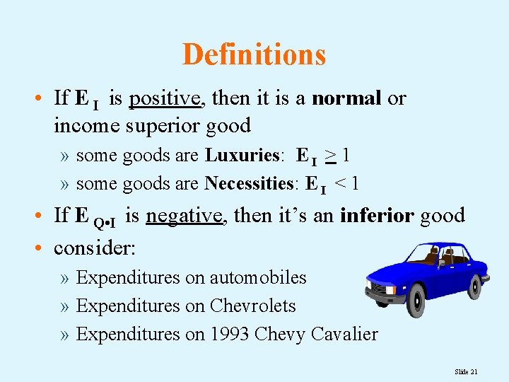
Definitions • If E I is positive, then it is a normal or income superior good » some goods are Luxuries: E I > 1 » some goods are Necessities: E I < 1 • If E Q • I is negative, then it’s an inferior good • consider: » Expenditures on automobiles » Expenditures on Chevrolets » Expenditures on 1993 Chevy Cavalier Slide 21

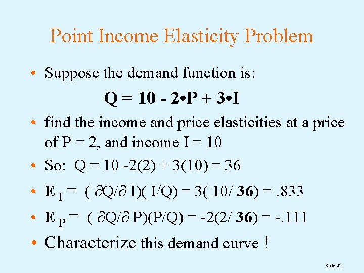
Point Income Elasticity Problem • Suppose the demand function is: Q = 10 - 2 • P + 3 • I • find the income and price elasticities at a price of P = 2, and income I = 10 • So: Q = 10 -2(2) + 3(10) = 36 • E I = ( Q/ I)( I/Q) = 3( 10/ 36) =. 833 • E P = ( Q/ P)(P/Q) = -2(2/ 36) = -. 111 • Characterize this demand curve ! Slide 22

Cross Price Elasticities E X = % Qx / % Py = ( Qx/ Py)(Py / Qx) • Substitutes have positive cross price elasticities: Butter & Margarine • Complements have negative cross price elasticities: VCR machines and the rental price of tapes • When the cross price elasticity is zero or insignificant, the products are not related Slide 23

HOMEWORK PROBLEM: Find the point price elasticity, the point income elasticity, and the point cross-price elasticity at P=10, I=20, and Ps=9, if the demand function were estimated to be: Qd = 90 - 8·P + 2·I + 2·Ps. Is the demand for this product elastic or inelastic? Is it a luxury or a necessity? Does this product have a close substitute or complement? Find the point elasticities of demand. Slide 24

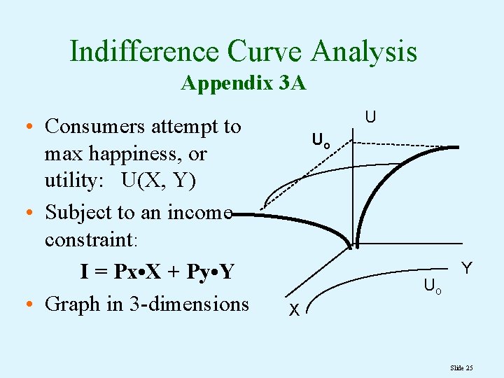
Indifference Curve Analysis Appendix 3 A • Consumers attempt to max happiness, or utility: U(X, Y) • Subject to an income constraint: I = Px • X + Py • Y • Graph in 3 -dimensions U Uo Uo Y X Slide 25

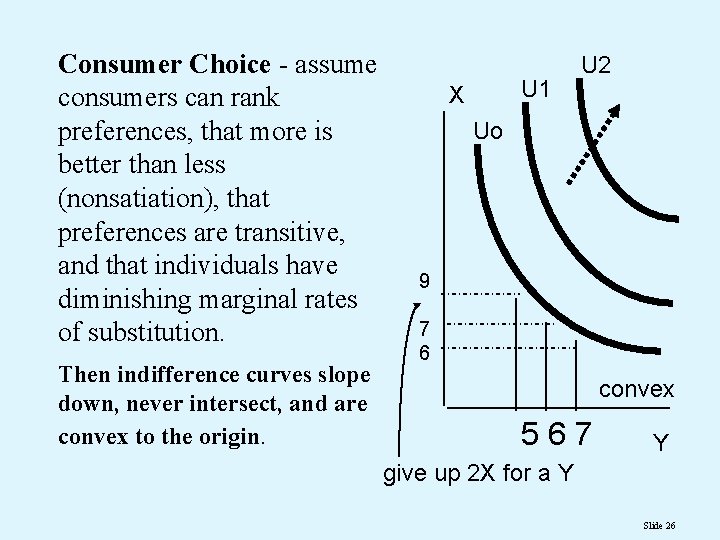
Consumer Choice - assume consumers can rank preferences, that more is better than less (nonsatiation), that preferences are transitive, and that individuals have diminishing marginal rates of substitution. Then indifference curves slope down, never intersect, and are convex to the origin. U 1 X U 2 Uo 9 7 6 convex 567 Y give up 2 X for a Y Slide 26

Uo U 1 X Indifference Curves a c b Y Py demand • We can "derive" a demand curve graphically from maximization of utility subject to a budget constraint. As price falls, we tend to buy more due to (i) the Income Effect and (ii) the Substitution Effect. Y Slide 27

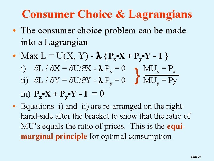
Consumer Choice & Lagrangians • The consumer choice problem can be made into a Lagrangian • Max L = U(X, Y) - {Px • X + Py • Y - I } i) L / X = U/ X - Px = 0 ii) L / Y = U/ Y - Py = 0 } MUx = Px MUy = Py iii) Px • X + Py • Y - I = 0 • Equations i) and ii) are re-arranged on the righthand-side after the bracket to show that the ratio of MU’s equals the ratio of prices. This is the equimarginal principle for optimal consumption Slide 28

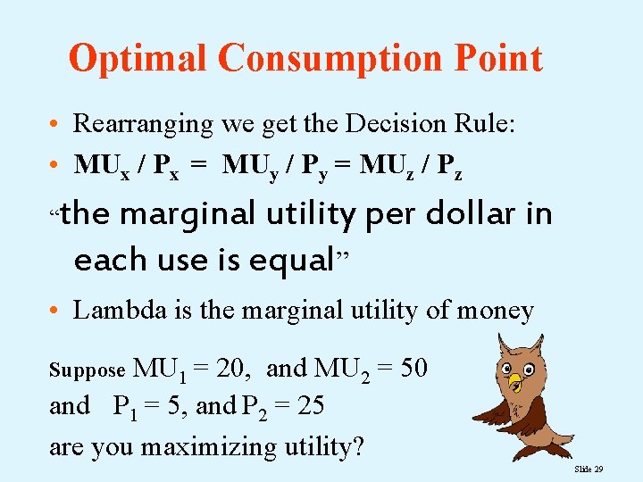
Optimal Consumption Point • Rearranging we get the Decision Rule: • MUx / Px = MUy / Py = MUz / Pz “ the marginal utility per dollar in each use is equal” • Lambda is the marginal utility of money MU 1 = 20, and MU 2 = 50 and P 1 = 5, and P 2 = 25 are you maximizing utility? Suppose Slide 29

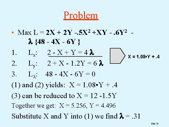
Problem • Max L = 2 X + 2 Y -. 5 X 2 +XY -. 6 Y 2 {48 - 4 X - 6 Y } 1. Lx: 2 - X + Y = 4 X = 1. 08 • Y +. 4 2. Ly: 2 + X - 1. 2 Y = 6 3. L : 48 - 4 X - 6 Y = 0 (1) and (2) yields: X = 1. 08 • Y +. 4 (3) can be reduced to X = 12 -1. 5 Y Together we get: X = 5. 256, Y = 4. 496 Substitute X and Y into (1) we find =. 31 Slide 30