DEMAND ANALYSIS Overview of Chapter 3 Demand Relationships

DEMAND ANALYSIS Overview of Chapter 3 • • • Demand Relationships Demand Elasticities Income Elasticities Cross Elasticities of Demand Combined Effects of Elasticities 2005 South-Western Publishing Slide 1

Health Care & Cigarettes • Raising cigarette taxes reduces smoking » In Canada, $4 for a pack of cigarettes reduced smoking 38% in a decade • But cigarette taxes also helps fund health care initiatives » The issue then, should we find a tax rate that maximizes tax revenues? » Or a tax rate that reduces smoking? Slide 2

Demand Analysis • An important contributor to firm risk arises from sudden shifts in demand for the product or service. • Demand analysis serves two managerial objectives: (1) it provides the insights necessary for effective management of demand, and (2) it aids in forecasting sales and revenues. Slide 3

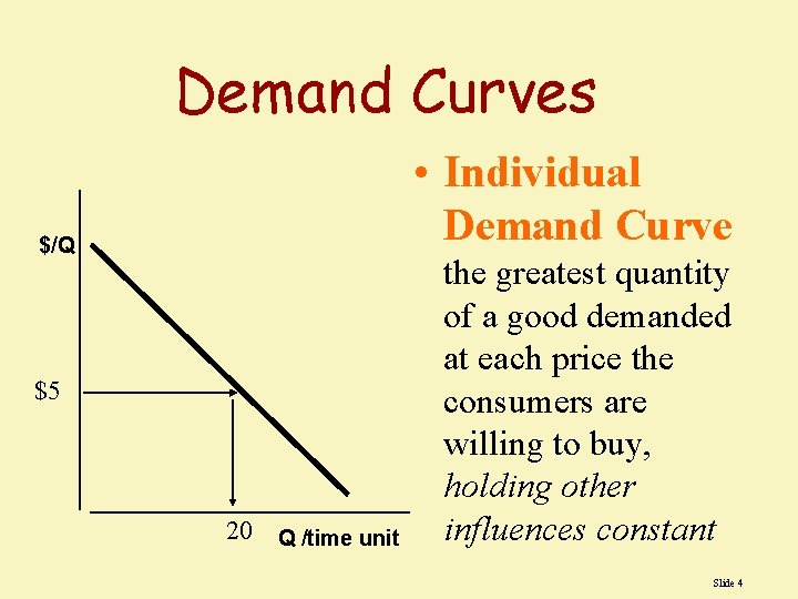
Demand Curves • Individual Demand Curve $/Q $5 20 Q /time unit the greatest quantity of a good demanded at each price the consumers are willing to buy, holding other influences constant Slide 4

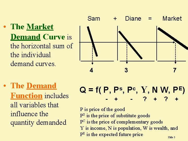
• The Market Demand Curve is the horizontal sum of the individual demand curves. • The Demand Function includes all variables that influence the quantity demanded Sam + 4 Diane = Market 3 7 Q = f( P, Ps, Pc, Y, N W, PE) - + - ? + P is price of the good PS is the price of substitute goods PC is the price of complementary goods Y is income, N is population, W is wealth, and PE is the expected future price Slide 5

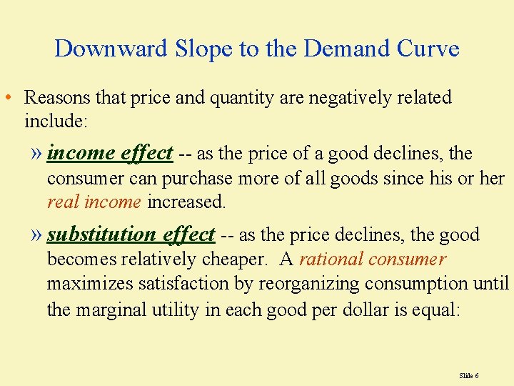
Downward Slope to the Demand Curve • Reasons that price and quantity are negatively related include: » income effect -- as the price of a good declines, the consumer can purchase more of all goods since his or her real income increased. » substitution effect -- as the price declines, the good becomes relatively cheaper. A rational consumer maximizes satisfaction by reorganizing consumption until the marginal utility in each good per dollar is equal: Slide 6

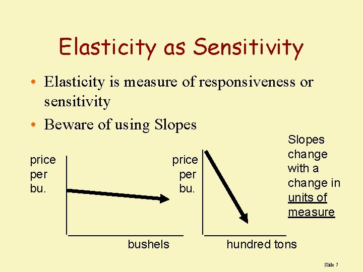
Elasticity as Sensitivity • Elasticity is measure of responsiveness or sensitivity • Beware of using Slopes price per bu. bushels Slopes change with a change in units of measure hundred tons Slide 7

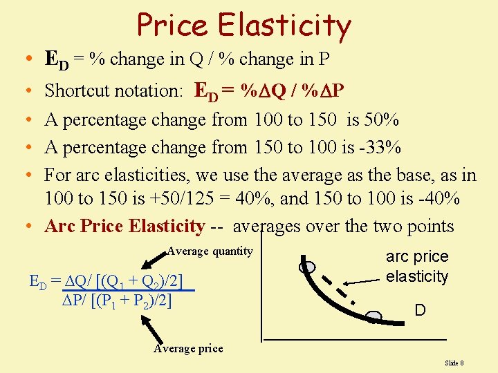
Price Elasticity • ED = % change in Q / % change in P • Shortcut notation: ED = % Q / % P • A percentage change from 100 to 150 is 50% • A percentage change from 150 to 100 is -33% • For arc elasticities, we use the average as the base, as in 100 to 150 is +50/125 = 40%, and 150 to 100 is -40% • Arc Price Elasticity -- averages over the two points Average quantity ED = Q/ [(Q 1 + Q 2)/2] P/ [(P 1 + P 2)/2] arc price elasticity D Average price Slide 8

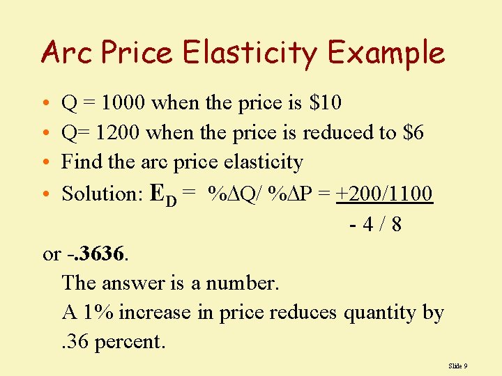
Arc Price Elasticity Example • • Q = 1000 when the price is $10 Q= 1200 when the price is reduced to $6 Find the arc price elasticity Solution: ED = % Q/ % P = +200/1100 -4/8 or -. 3636. The answer is a number. A 1% increase in price reduces quantity by. 36 percent. Slide 9

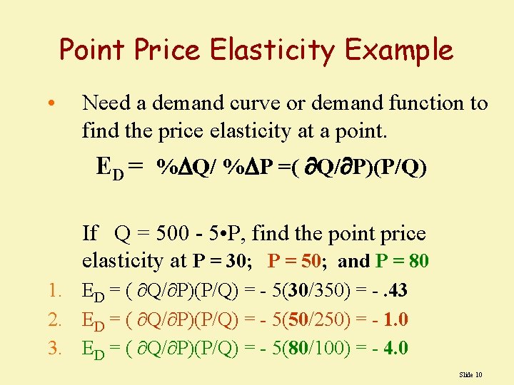
Point Price Elasticity Example • Need a demand curve or demand function to find the price elasticity at a point. ED = % Q/ % P =( Q/ P)(P/Q) If Q = 500 - 5 • P, find the point price elasticity at P = 30; P = 50; and P = 80 1. ED = ( Q/ P)(P/Q) = - 5(30/350) = -. 43 2. ED = ( Q/ P)(P/Q) = - 5(50/250) = - 1. 0 3. ED = ( Q/ P)(P/Q) = - 5(80/100) = - 4. 0 Slide 10

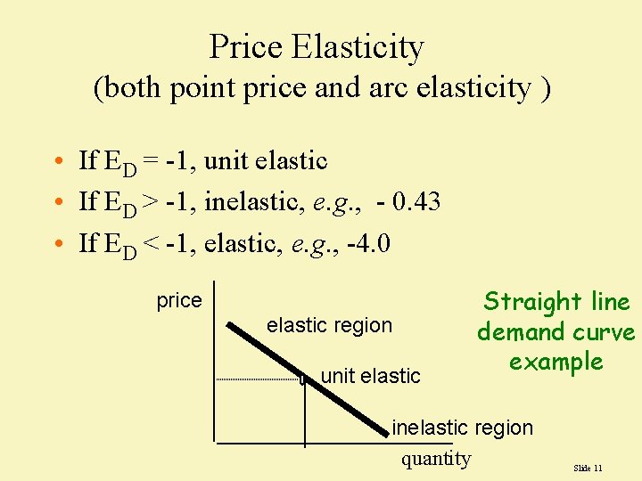
Price Elasticity (both point price and arc elasticity ) • If ED = -1, unit elastic • If ED > -1, inelastic, e. g. , - 0. 43 • If ED < -1, elastic, e. g. , -4. 0 price elastic region unit elastic Straight line demand curve example inelastic region quantity Slide 11

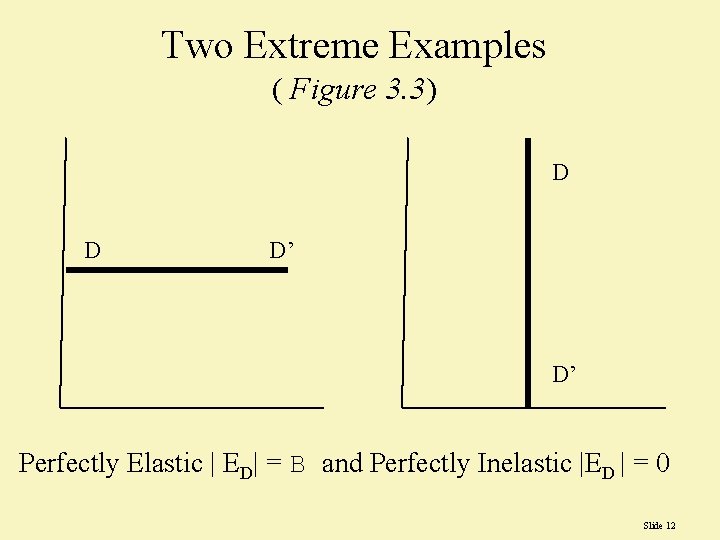
Two Extreme Examples ( Figure 3. 3) D D D’ D’ Perfectly Elastic | ED| = B and Perfectly Inelastic |ED | = 0 Slide 12

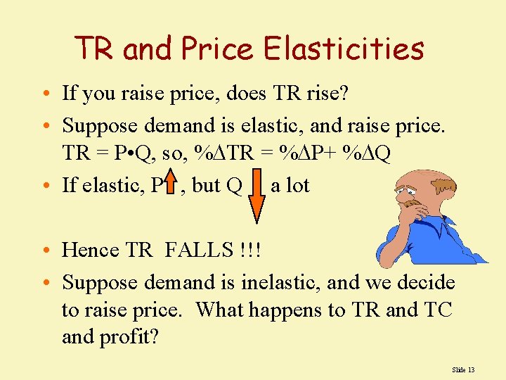
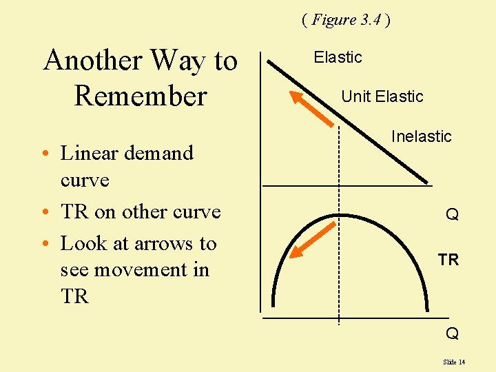
TR and Price Elasticities • If you raise price, does TR rise? • Suppose demand is elastic, and raise price. TR = P • Q, so, % TR = % P+ % Q • If elastic, P , but Q a lot • Hence TR FALLS !!! • Suppose demand is inelastic, and we decide to raise price. What happens to TR and TC and profit? Slide 13

( Figure 3. 4 ) Another Way to Remember • Linear demand curve • TR on other curve • Look at arrows to see movement in TR Elastic Unit Elastic Inelastic Q TR Q Slide 14

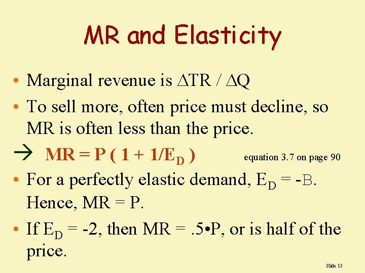
MR and Elasticity • Marginal revenue is TR / Q • To sell more, often price must decline, so MR is often less than the price. à MR = P ( 1 + 1/ED ) equation 3. 7 on page 90 • For a perfectly elastic demand, ED = -B. Hence, MR = P. • If ED = -2, then MR =. 5 • P, or is half of the price. Slide 15

1979 Deregulation of Airfares • • Prices declined after deregulation And passengers increased Also total revenue increased What does this imply about the price elasticity of air travel? » It must be that air travel was elastic, as a price decrease after deregulation led to greater total revenue for the airlines. Slide 16

Determinants of the Price Elasticity • The availability and the closeness of substitutes » more substitutes, more elastic • The more durable is the product » Durable goods are more elastic than non-durables • The percentage of the budget » larger proportion of the budget, more elastic • The longer the time period permitted » more time, generally, more elastic » consider examples of business travel versus vacation travel for all three above. Slide 17

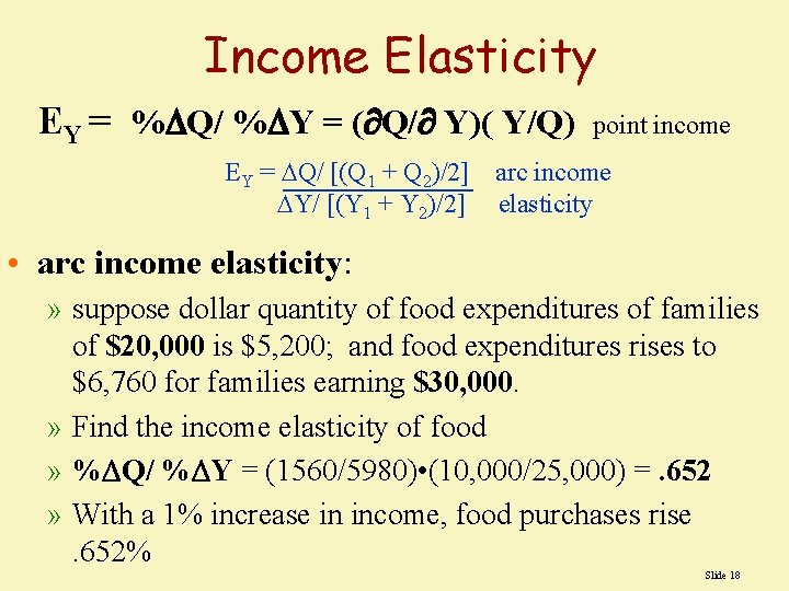
Income Elasticity EY = % Q/ % Y = ( Q/ Y)( Y/Q) point income EY = Q/ [(Q 1 + Q 2)/2] arc income Y/ [(Y 1 + Y 2)/2] elasticity • arc income elasticity: » suppose dollar quantity of food expenditures of families of $20, 000 is $5, 200; and food expenditures rises to $6, 760 for families earning $30, 000. » Find the income elasticity of food » % Q/ % Y = (1560/5980) • (10, 000/25, 000) =. 652 » With a 1% increase in income, food purchases rise. 652% Slide 18

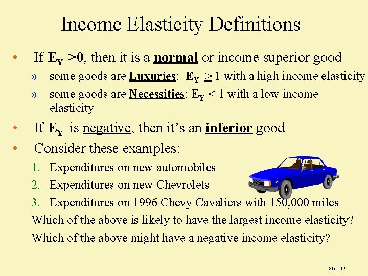
Income Elasticity Definitions • If EY >0, then it is a normal or income superior good » some goods are Luxuries: EY > 1 with a high income elasticity » some goods are Necessities: EY < 1 with a low income elasticity • • If EY is negative, then it’s an inferior good Consider these examples: 1. Expenditures on new automobiles 2. Expenditures on new Chevrolets 3. Expenditures on 1996 Chevy Cavaliers with 150, 000 miles Which of the above is likely to have the largest income elasticity? Which of the above might have a negative income elasticity? Slide 19

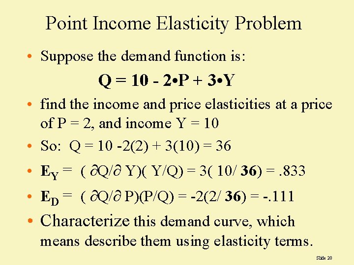
Point Income Elasticity Problem • Suppose the demand function is: Q = 10 - 2 • P + 3 • Y • find the income and price elasticities at a price of P = 2, and income Y = 10 • So: Q = 10 -2(2) + 3(10) = 36 • EY = ( Q/ Y)( Y/Q) = 3( 10/ 36) =. 833 • ED = ( Q/ P)(P/Q) = -2(2/ 36) = -. 111 • Characterize this demand curve, which means describe them using elasticity terms. Slide 20

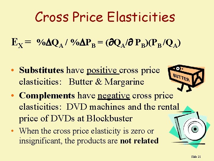
Cross Price Elasticities EX = % QA / % PB = ( QA/ PB)(PB /QA) • Substitutes have positive cross price elasticities: Butter & Margarine • Complements have negative cross price elasticities: DVD machines and the rental price of DVDs at Blockbuster • When the cross price elasticity is zero or insignificant, the products are not related Slide 21

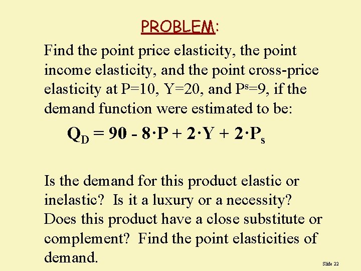
PROBLEM: Find the point price elasticity, the point income elasticity, and the point cross-price elasticity at P=10, Y=20, and Ps=9, if the demand function were estimated to be: QD = 90 - 8·P + 2·Y + 2·Ps Is the demand for this product elastic or inelastic? Is it a luxury or a necessity? Does this product have a close substitute or complement? Find the point elasticities of demand. Slide 22

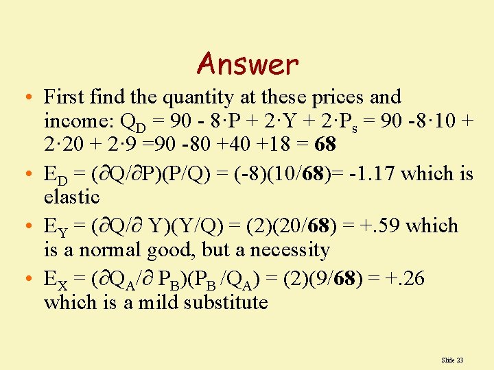
Answer • First find the quantity at these prices and income: QD = 90 - 8·P + 2·Y + 2·Ps = 90 -8· 10 + 2· 20 + 2· 9 =90 -80 +40 +18 = 68 • ED = ( Q/ P)(P/Q) = (-8)(10/68)= -1. 17 which is elastic • EY = ( Q/ Y)(Y/Q) = (2)(20/68) = +. 59 which is a normal good, but a necessity • EX = ( QA/ PB)(PB /QA) = (2)(9/68) = +. 26 which is a mild substitute Slide 23

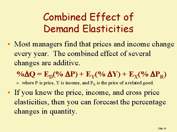
Combined Effect of Demand Elasticities • Most managers find that prices and income change every year. The combined effect of several changes are additive. % Q = ED(% P) + EY(% Y) + EX(% PR) » where P is price, Y is income, and PR is the price of a related good. • If you knew the price, income, and cross price elasticities, then you can forecast the percentage changes in quantity. Slide 24

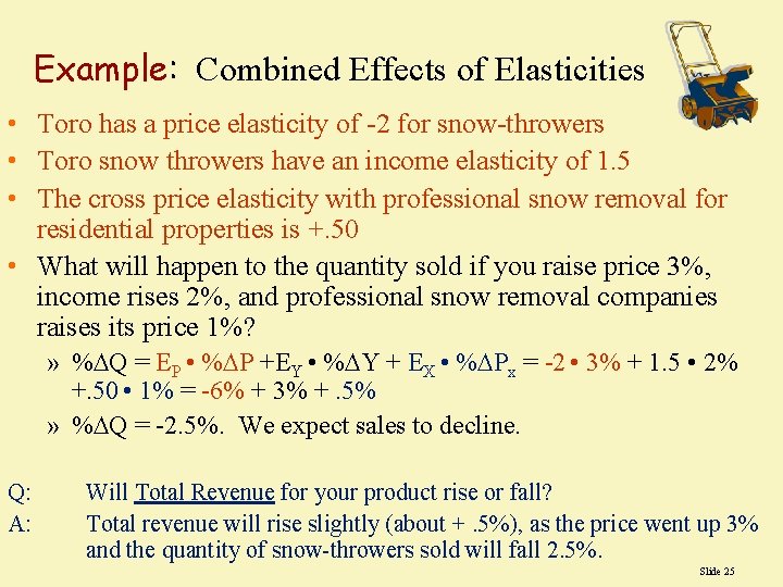
Example: Combined Effects of Elasticities • Toro has a price elasticity of -2 for snow-throwers • Toro snow throwers have an income elasticity of 1. 5 • The cross price elasticity with professional snow removal for residential properties is +. 50 • What will happen to the quantity sold if you raise price 3%, income rises 2%, and professional snow removal companies raises its price 1%? » % Q = EP • % P +EY • % Y + EX • % Px = -2 • 3% + 1. 5 • 2% +. 50 • 1% = -6% + 3% +. 5% » % Q = -2. 5%. We expect sales to decline. Q: A: Will Total Revenue for your product rise or fall? Total revenue will rise slightly (about +. 5%), as the price went up 3% and the quantity of snow-throwers sold will fall 2. 5%. Slide 25