Delaunay Triangulation Based WideArea Visualization of Electric Transmission

Delaunay Triangulation Based Wide-Area Visualization of Electric Transmission Grids Thomas J. Overbye, Jess Wert, Komal S. Shetye, Farnaz Safdarian, Adam B. Birchfield Texas A&M University overbye@tamu. edu Kansas Power and Energy Conference April 19 -20, 2021

Background: Engineering Models • All models are wrong but some are useful, “ – George Box, Empirical Model-Building and Response Surfaces, (1987, p. 424) (also in his 1976 paper) – He was a professor at UW-Madison from 1960 onwards, forming their Department of Statistics. He died in 2013 and UW-Madison recently had a George Box Centenary Celebration; he has 195, 000 google scholar citations!! – Box went on to comment on the need to consider the degree of wrongness and when models stop being useful – The math itself is not wrong • This applies throughout engineering including with visualizations. We need to focus on usefulness!! 2

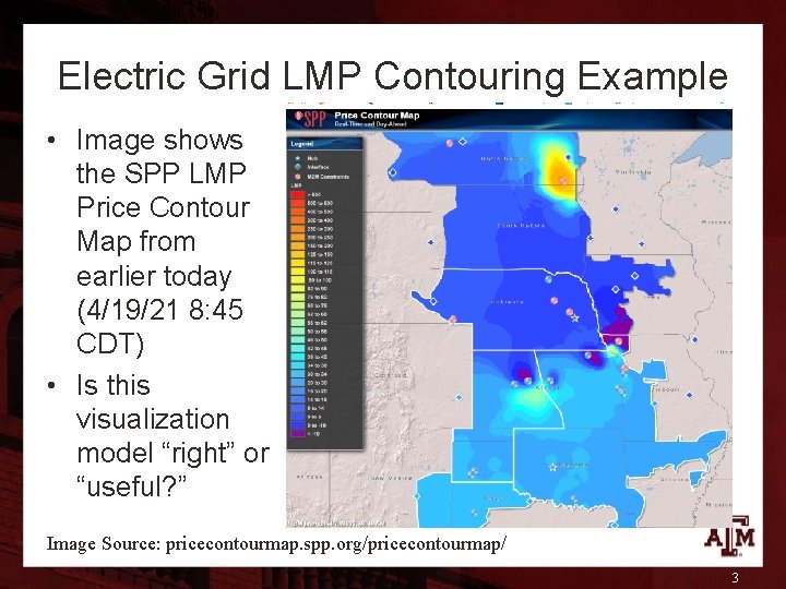
Electric Grid LMP Contouring Example • Image shows the SPP LMP Price Contour Map from earlier today (4/19/21 8: 45 CDT) • Is this visualization model “right” or “useful? ” Image Source: pricecontourmap. spp. org/pricecontourmap/ 3

History of Power System Contouring • Contouring was first proposed in mid 1990’s but dismissed as not being useful • In late 1990’s Jamie Weber and I independently applied contouring to electric grid information – First presented at NAPS 1997 (the blizzard NAPS) and later published in a 2000 IEEE Trans. Power Sys. Paper • In the papers we argued that contouring was wrong but that is usefulness outweighed its wrongness – It is wrong because 1) power system data is discrete not continuous, 2) LTCs (and congestion) introduce discrete changes in the values, 3) electric values near on the contour might be quite distant electrically • It is wrong (like all models) but it is now widely used 4

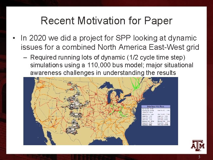
Recent Motivation for Paper • In 2020 we did a project for SPP looking at dynamic issues for a combined North America East-West grid – Required running lots of dynamic (1/2 cycle time step) simulations using a 110, 000 bus model; major situational awareness challenges in understanding the results 5

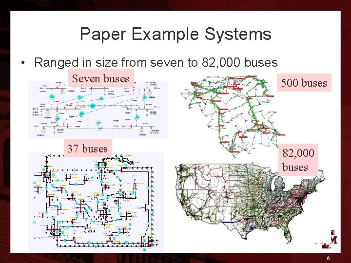
Paper Example Systems • Ranged in size from seven to 82, 000 buses Seven buses 37 buses 500 buses 82, 000 buses 6

Power System Visualization • There are several different ways for showing power system information and they are complimentary – Tabular displays: these can be very useful, particularly with interactive capabilities like filtering, sorting, drill-down – Graphical visualizations including onelines: they come with many different variations, though typically it is easiest to visualization bus-based Image shows US generators by location, information size and fuel type; based on EIA-860 data – Geographic data views are very useful! – Flow information is harder: “Can’t see the forest for the trees. ” 7

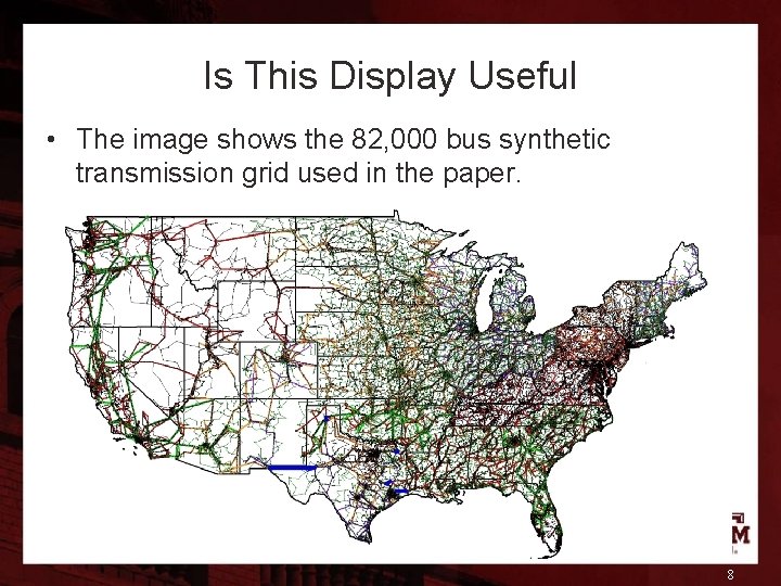
Is This Display Useful • The image shows the 82, 000 bus synthetic transmission grid used in the paper. 8

Paper’s Contribution • The key contributions of the paper are 1) an algorithm for visualizing power system flows using a Delaunay triangulation approach (giving a planar graph), 2) an algorithm demonstration on grids of all sizes, different levels of aggregation and different flows • The algorithm is simple and fast – Assume n buses, m bus groups and b branches joining the buses, with geographic information available for the buses – Map each branch to its terminal bus group(s) – Do a Delaunay triangulation of the m bus groups to create a set S of segments – For each branch quickly determine a segment path between its terminal bus groups adding it to the list for each segment 9

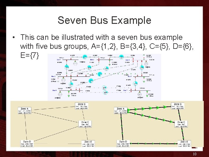
Seven Bus Example • This can be illustrated with a seven bus example with five bus groups, A={1, 2}, B={3, 4}, C={5}, D={6}, E={7} 10

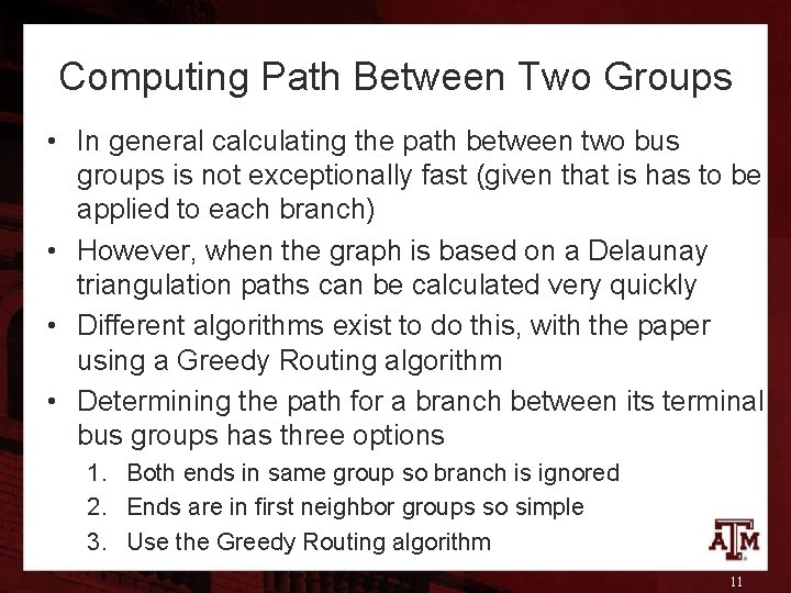
Computing Path Between Two Groups • In general calculating the path between two bus groups is not exceptionally fast (given that is has to be applied to each branch) • However, when the graph is based on a Delaunay triangulation paths can be calculated very quickly • Different algorithms exist to do this, with the paper using a Greedy Routing algorithm • Determining the path for a branch between its terminal bus groups has three options 1. Both ends in same group so branch is ignored 2. Ends are in first neighbor groups so simple 3. Use the Greedy Routing algorithm 11

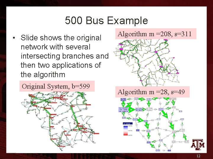
500 Bus Example • Slide shows the original network with several intersecting branches and then two applications of the algorithm Original System, b=599 Algorithm m =208, s=311 Algorithm m =28, s=49 12

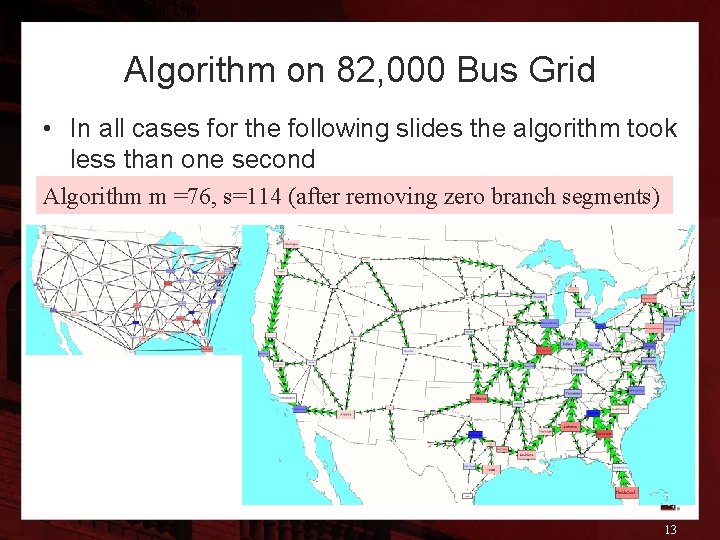
Algorithm on 82, 000 Bus Grid • In all cases for the following slides the algorithm took less than one second Algorithm m =76, s=114 (after removing zero branch segments) 13

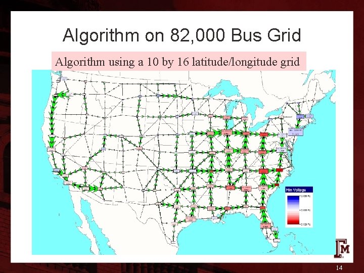
Algorithm on 82, 000 Bus Grid Algorithm using a 10 by 16 latitude/longitude grid 14

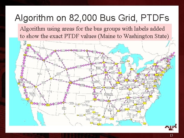
Algorithm on 82, 000 Bus Grid, PTDFs Algorithm using areas for the bus groups with labels added to show the exact PTDF values (Maine to Washington State) 15

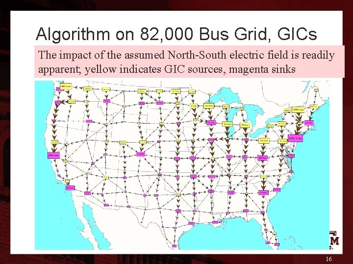
Algorithm on 82, 000 Bus Grid, GICs The impact of the assumed North-South electric field is readily apparent; yellow indicates GIC sources, magenta sinks 16

Thank You! Questions? Also, please join us in person at Texas A&M for NAPS 2021 on November 14 -16 in College Station, with papers due July 15, 2021 17