Defining Efficiency Asymptotic Complexity how running time scales

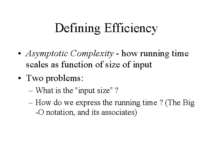
Defining Efficiency • Asymptotic Complexity - how running time scales as function of size of input • Two problems: – What is the “input size” ? – How do we express the running time ? (The Big -O notation, and its associates)

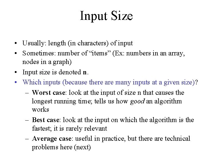
Input Size • Usually: length (in characters) of input • Sometimes: number of “items” (Ex: numbers in an array, nodes in a graph) • Input size is denoted n. • Which inputs (because there are many inputs at a given size)? – Worst case: look at the input of size n that causes the longest running time; tells us how good an algorithm works – Best case: look at the input on which the algorithm is the fastest; it is rarely relevant – Average case: useful in practice, but there are technical problems here (next)

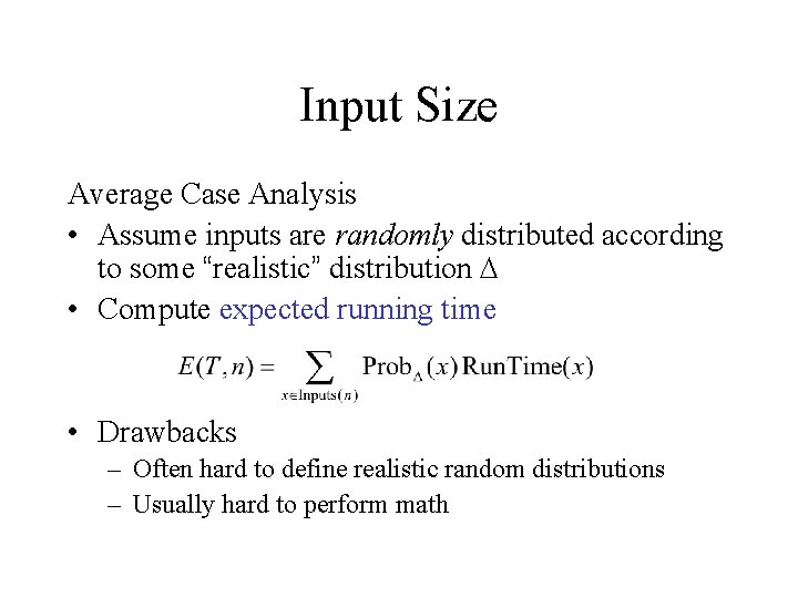
Input Size Average Case Analysis • Assume inputs are randomly distributed according to some “realistic” distribution • Compute expected running time • Drawbacks – Often hard to define realistic random distributions – Usually hard to perform math

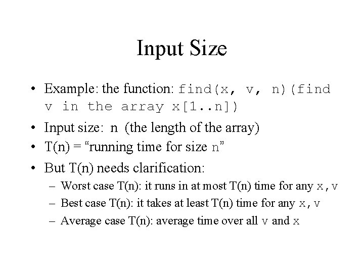
Input Size • Example: the function: find(x, v, n)(find v in the array x[1. . n]) • Input size: n (the length of the array) • T(n) = “running time for size n” • But T(n) needs clarification: – Worst case T(n): it runs in at most T(n) time for any x, v – Best case T(n): it takes at least T(n) time for any x, v – Average case T(n): average time over all v and x

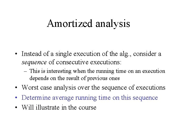
Amortized analysis • Instead of a single execution of the alg. , consider a sequence of consecutive executions: – This is interesting when the running time on an execution depends on the result of previous ones • Worst case analysis over the sequence of executions • Determine average running time on this sequence • Will illustrate in the course

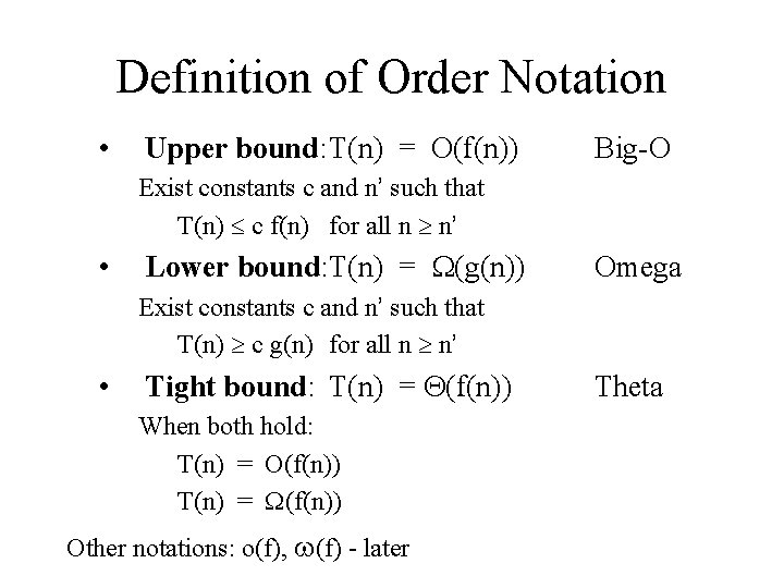
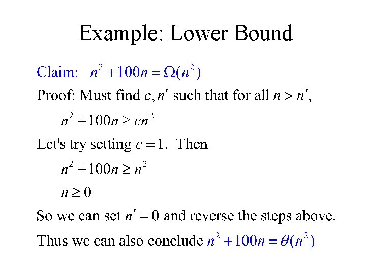
Definition of Order Notation • Upper bound: T(n) = O(f(n)) Big-O Exist constants c and n’ such that T(n) c f(n) for all n n’ • Lower bound: T(n) = (g(n)) Omega Exist constants c and n’ such that T(n) c g(n) for all n n’ • Tight bound: T(n) = (f(n)) When both hold: T(n) = O(f(n)) T(n) = (f(n)) Other notations: o(f), (f) - later Theta

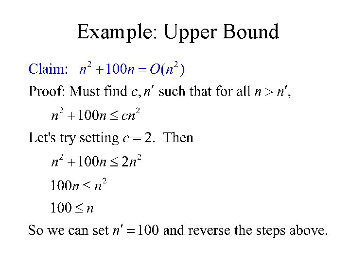
Example: Upper Bound

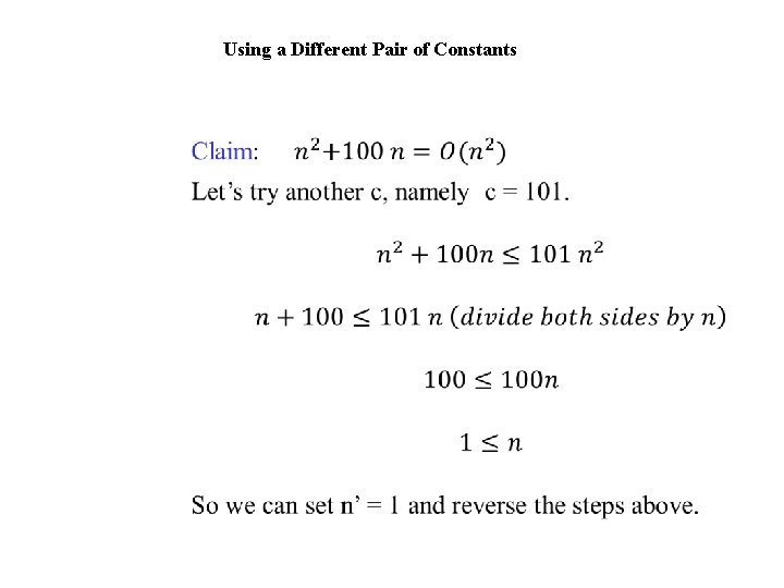
Using a Different Pair of Constants

Example: Lower Bound

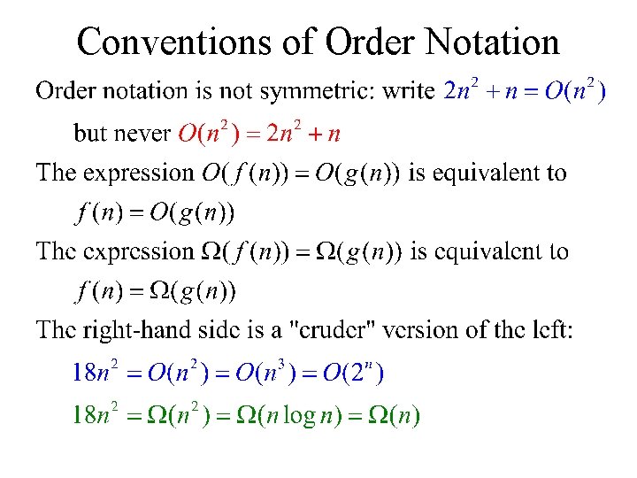
Conventions of Order Notation

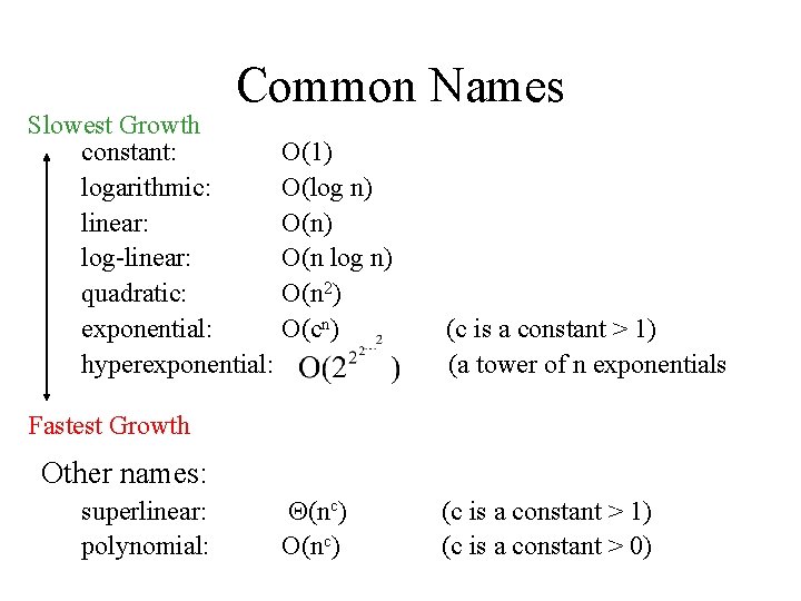
Common Names Slowest Growth constant: O(1) logarithmic: O(log n) linear: O(n) log-linear: O(n log n) quadratic: O(n 2) exponential: O(cn) (c is a constant > 1) hyperexponential: (a tower of n exponentials Fastest Growth Other names: superlinear: polynomial: (nc) O(nc) (c is a constant > 1) (c is a constant > 0)

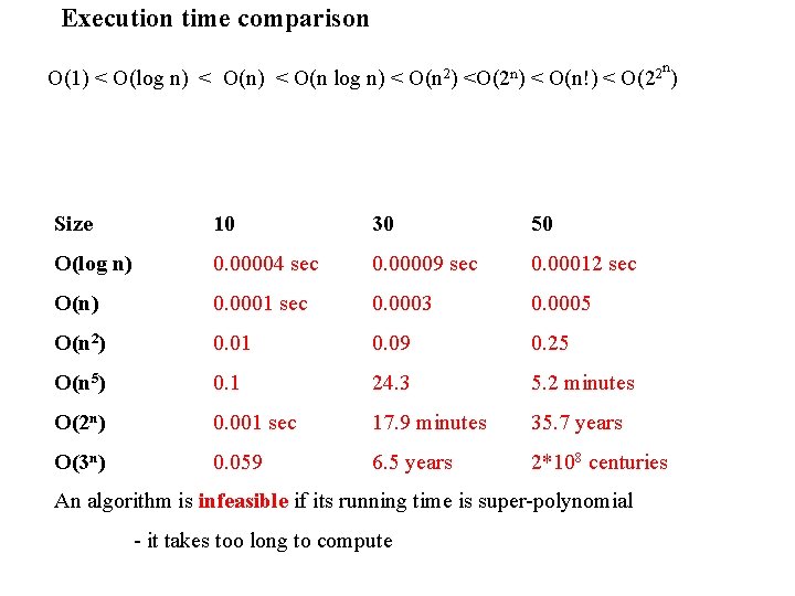
Execution time comparison n O(1) < O(log n) < O(n 2) <O(2 n) < O(n!) < O(22 ) Size 10 30 50 O(log n) 0. 00004 sec 0. 00009 sec 0. 00012 sec O(n) 0. 0001 sec 0. 0003 0. 0005 O(n 2) 0. 01 0. 09 0. 25 O(n 5) 0. 1 24. 3 5. 2 minutes O(2 n) 0. 001 sec 17. 9 minutes 35. 7 years O(3 n) 0. 059 6. 5 years 2*108 centuries An algorithm is infeasible if its running time is super-polynomial - it takes too long to compute

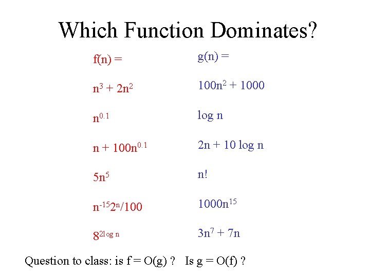
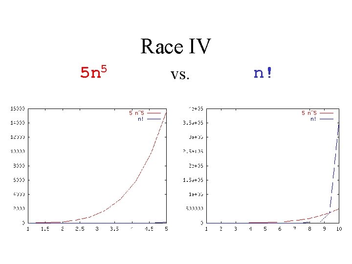
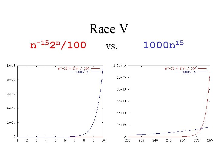
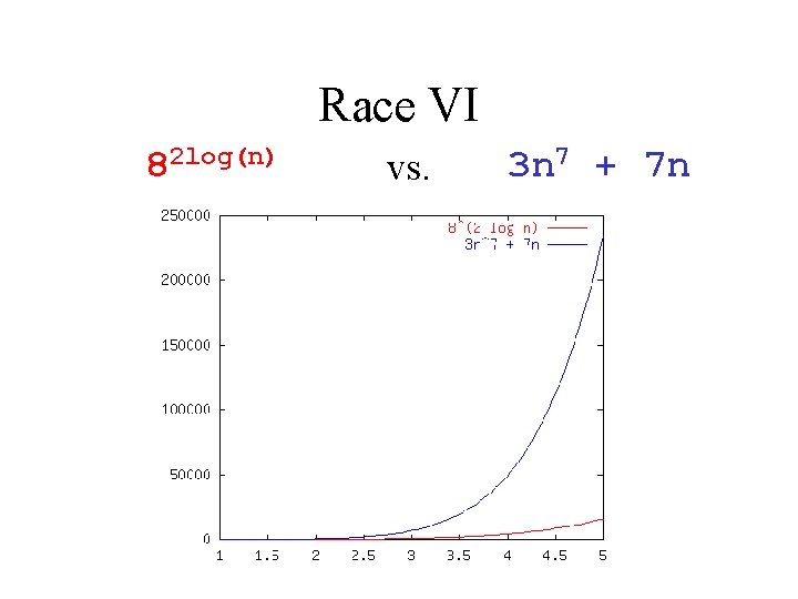
Which Function Dominates? f(n) = g(n) = n 3 + 2 n 2 100 n 2 + 1000 n 0. 1 log n n + 100 n 0. 1 2 n + 10 log n 5 n 5 n! n-152 n/100 1000 n 15 82 log n 3 n 7 + 7 n Question to class: is f = O(g) ? Is g = O(f) ?

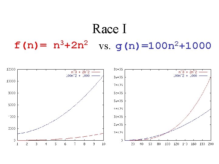
Race I f(n)= n 3+2 n 2 vs. g(n)=100 n 2+1000

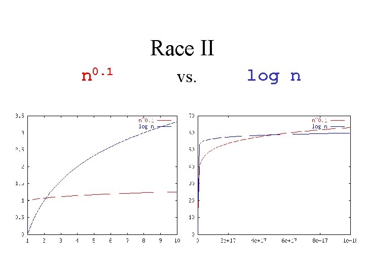
Race II n 0. 1 vs. log n

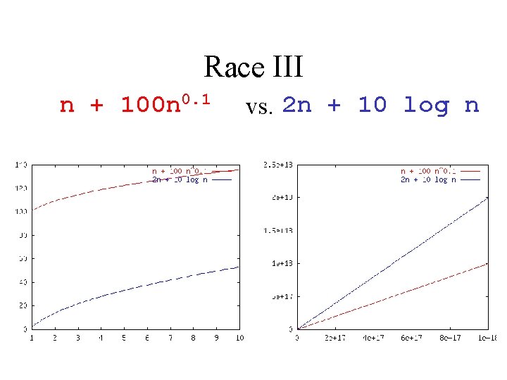
Race III n + 100 n 0. 1 vs. 2 n + 10 log n

Race IV 5 n 5 vs. n!

Race V n-152 n/100 vs. 1000 n 15

Race VI 82 log(n) vs. 3 n 7 + 7 n

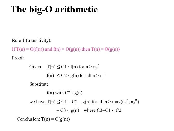
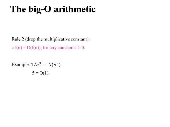
The big-O arithmetic

The big-O arithmetic

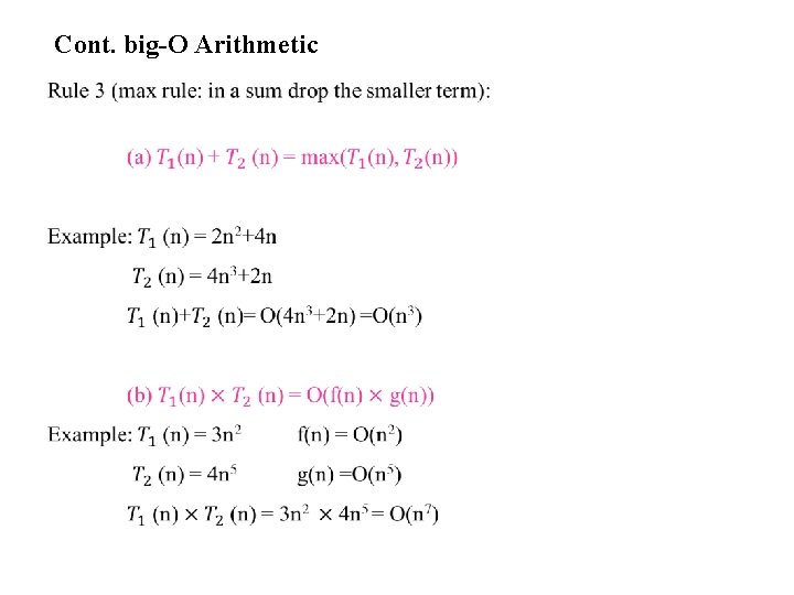
Cont. big-O Arithmetic

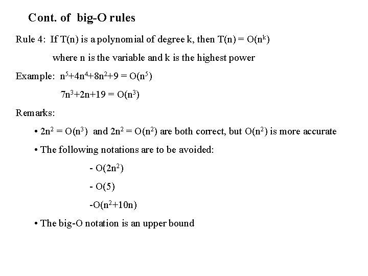
Cont. of big-O rules Rule 4: If T(n) is a polynomial of degree k, then T(n) = O(nk) where n is the variable and k is the highest power Example: n 5+4 n 4+8 n 2+9 = O(n 5) 7 n 3+2 n+19 = O(n 3) Remarks: • 2 n 2 = O(n 3) and 2 n 2 = O(n 2) are both correct, but O(n 2) is more accurate • The following notations are to be avoided: - O(2 n 2) - O(5) -O(n 2+10 n) • The big-O notation is an upper bound

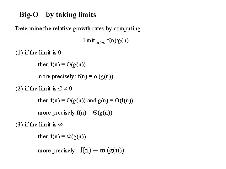
Big-O – by taking limits Determine the relative growth rates by computing limit n-> f(n)/g(n) (1) if the limit is 0 then f(n) = O(g(n)) more precisely: f(n) = o (g(n)) (2) if the limit is C 0 then f(n) = O(g(n)) and g(n) = O(f(n)) more precisely f(n) = (g(n)) (3) if the limit is then f(n) = (g(n)) more precisely: f(n) = (g(n))

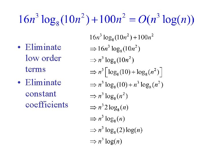
• Eliminate low order terms • Eliminate constant coefficients

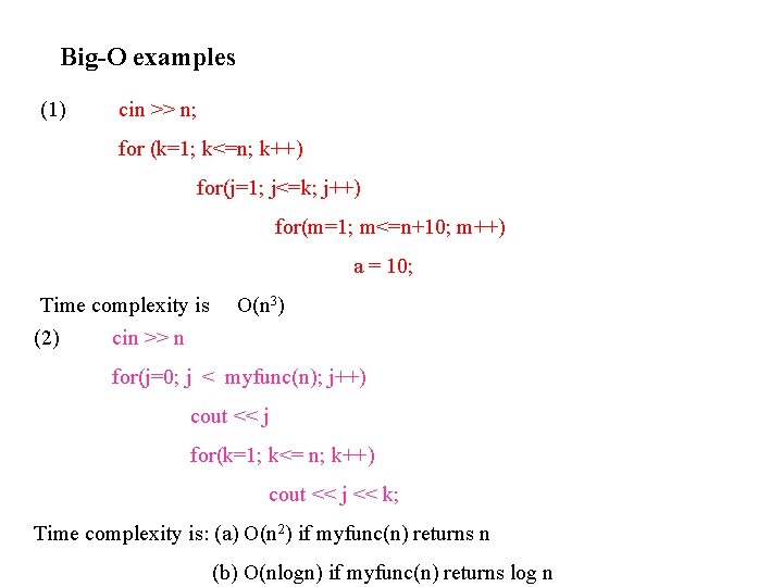
Big-O examples (1) cin >> n; for (k=1; k<=n; k++) for(j=1; j<=k; j++) for(m=1; m<=n+10; m++) a = 10; Time complexity is O(n 3) (2) cin >> n for(j=0; j < myfunc(n); j++) cout << j for(k=1; k<= n; k++) cout << j << k; Time complexity is: (a) O(n 2) if myfunc(n) returns n (b) O(nlogn) if myfunc(n) returns log n

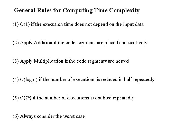
General Rules for Computing Time Complexity (1) O(1) if the execution time does not depend on the input data (2) Apply Addition if the code segments are placed consecutively (3) Apply Multiplication if the code segments are nested (4) O(log n) if the number of executions is reduced in half repeatedly (5) O(2 n) if the number of executions is doubled repeatedly (6) Always consider the worst case

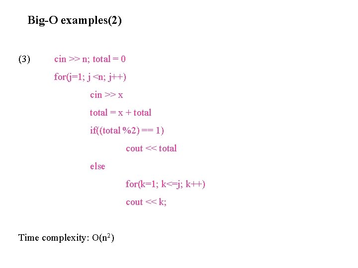
Big-O examples(2) (3) cin >> n; total = 0 for(j=1; j <n; j++) cin >> x total = x + total if((total %2) == 1) cout << total else for(k=1; k<=j; k++) cout << k; Time complexity: O(n 2)

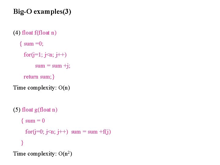
Big-O examples(3) (4) float f(float n) { sum =0; for(j=1; j<n; j++) sum = sum +j; return sum; } Time complexity: O(n) (5) float g(float n) { sum = 0 for(j=0; j<n; j++) sum = sum +f(j) } Time complexity: O(n 2)

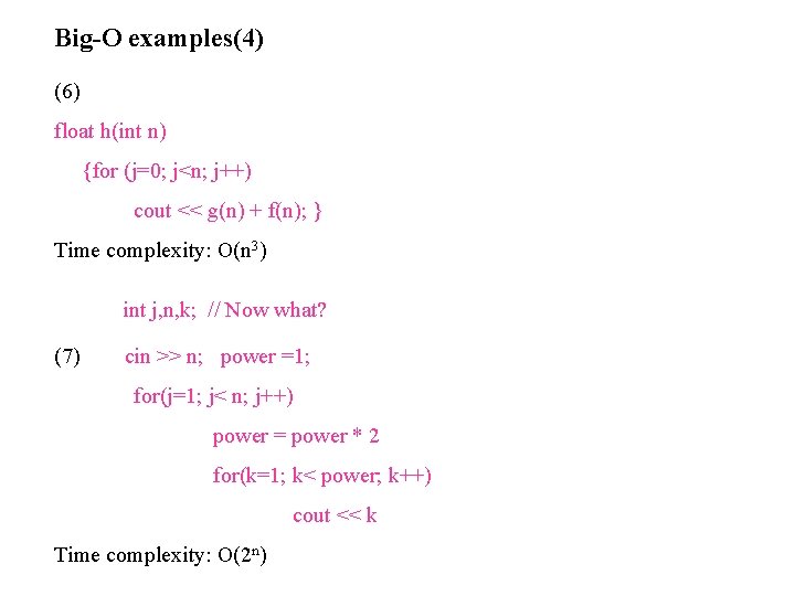
Big-O examples(4) (6) float h(int n) {for (j=0; j<n; j++) cout << g(n) + f(n); } Time complexity: O(n 3) int j, n, k; // Now what? (7) cin >> n; power =1; for(j=1; j< n; j++) power = power * 2 for(k=1; k< power; k++) cout << k Time complexity: O(2 n)

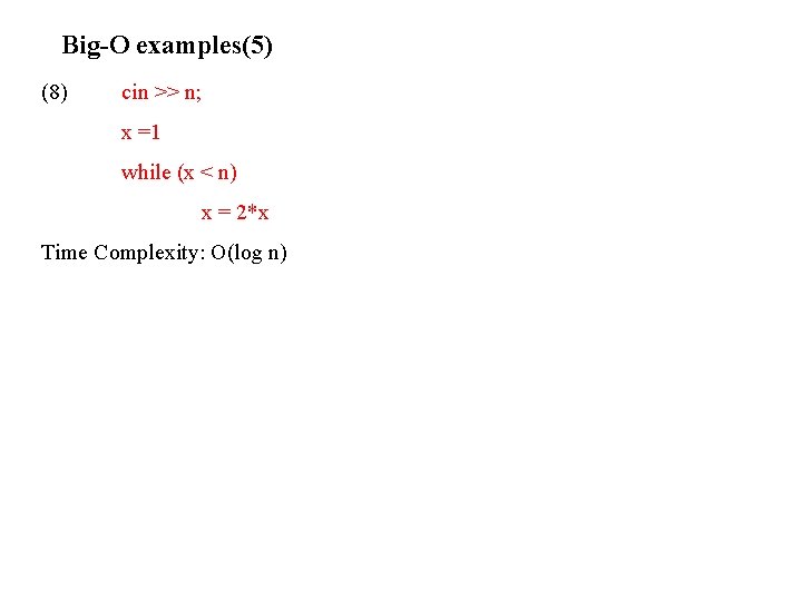
Big-O examples(5) (8) cin >> n; x =1 while (x < n) x = 2*x Time Complexity: O(log n)