Deep Sea Coral Predictive Habitat Suitability Model for

Deep Sea Coral Predictive Habitat Suitability Model for the U. S. Northeast and Mid-Atlantic Regions Brian Kinlan, Matthew Poti, Dan Dorfman, Chris Caldow NATIONAL OCEAN SERVICE National Centers for Coastal Ocean Science Amy Drohan, Dave Packer, Martha Nizinski Citation: Kinlan BP, Poti M, Drohan A, Packer DB, Nizinski M, Dorfman D, Caldow C. 2013. Digital data: Predictive models of deep-sea coral habitat suitability in the U. S. Northeast Atlantic and Mid-Atlantic regions. Downloadable digital data package. Department of Commerce (DOC), National Oceanic and Atmospheric Administration (NOAA), National Ocean Service (NOS), National Centers for Coastal Ocean Science (NCCOS), Center for Coastal Monitoring and Assessment (CCMA), Biogeography Branch. Released August 2013.

Deep-Sea Corals • • Diverse and valuable resource Important providers of habitat structure for fishes and invertebrates Conservation concern o slow growth rates o vulnerability to bottom disturbance Need for spatially explicit information on coral distribution o Deep sea surveys are logistically difficult and expensive Conger eel and squat lobster in Lophelia reefs. Photo Credit: S. Ross et al.

Value of Modeling • Conservation planning • Ecosystem-based fishery management • Siting and environmental impact assessment for offshore activities (e. g. , renewable energy) • Planning and targeting mapping and exploration efforts • Insights into environmental factors driving distribution of deep-sea corals

2011 -2013 DSC Modeling Efforts Region Northeast Southeast Gulf of Mexico Modeling complete June 2012 October 2012 February 2013 Publications/Data products complete May 2013 June 2013 July 2013
 Bathymetry: NOAA 3 arc-second Coastal Relief Model")
Northeast Study Area (New England & Mid-Atlantic) Bathymetry: NOAA 3 arc-second Coastal Relief Model (CRM) Depth (meters)
 predictive habitat models o Machine-learning technique o")
Modeling Approach • Maximum Entropy (Max. Ent) predictive habitat models o Machine-learning technique o Widely used for presence-only data o Software: Max. Ent version 3. 3. 3 k http: //www. cs. princeton. edu/~schapire/maxent Phillips et al. (2004) Proc Intl Conf Machine Learning Phillips et al. (2006) Ecological Modelling Phillips and Dudik (2008) Ecography Elith et al. (2011) Diversity and Distributions • • Models the relationship between two types of data: Known deep-sea coral presences Environmental predictor variables 1. 2. Caveat: Model outputs will reflect sampling biases

Model Input Data • Deep sea coral presence records acquired from National Deep-Sea Coral Geodatabase (NOAA DSCRTP 2012) from variety of historical sources (Packer et al. 2007, Scanlon et al. 2010, Packer and Dorfman 2012, Packer and Drohan 2012) Alcyonacea Pennatulacea Scleractinia

Northeast: Modeled deep-sea coral taxonomic groups Region Group Description Northeast U. S. 1 a Northeast U. S. 1 b 2 Northeast U. S. 2 a Family Caryophylliidae Northeast U. S. 2 b Family Flabellidae Northeast U. S. 3 Order Pennatulacea Northeast U. S. 3 a 3 b Order Alcyonacea Gorgonian Alcyonacea (Suborders Calcaxonia, Holaxonia, Scleraxonia) Non-Gorgonian Alcyonacea (Suborders Alcyoniina, Stolonifera) Order Scleractinia Suborder Sessiliflorae Suborder Subsessiliflorae Code name ALCY-GORG ALCY-NONGORG SCLER-CARYO SCLER-FLAB PENN-SESS PENN-SUBSESS

Northeast: Modeled deep-sea coral taxonomic groups Region Group Description Northeast U. S. 1 a Northeast U. S. 1 b 2 Northeast U. S. 2 a Family Caryophylliidae Northeast U. S. 2 b Family Flabellidae Northeast U. S. 3 Order Pennatulacea Northeast U. S. 3 a 3 b Order Alcyonacea Gorgonian Alcyonacea (Suborders Calcaxonia, Holaxonia, Scleraxonia) Non-Gorgonian Alcyonacea (Suborders Alcyoniina, Stolonifera) Order Scleractinia Suborder Sessiliflorae Suborder Subsessiliflorae Code name ALCY-GORG ALCY-NONGORG SCLER-CARYO SCLER-FLAB PENN-SESS PENN-SUBSESS

Model Input Data • Environmental predictor variables • • Terrain, Substrate, Physical & Biological Oceanography Processed to 370 meter horizontal grid resolution Terrain features analyzed at multiple scales: 370 m, 1. 5 km, 10 km, 20 km (Finer scale seafloor features not resolved by this regional model) Highly correlated variables eliminated and initial list of 64 potential predictor variables narrowed to 22. Final models selected variables from this list of 22:
 Annual Mean Bottom Salinity")
Predictor variable gallery Depth Bathymetric Position/Slope Index Aspect (5 km) Annual Mean Bottom Salinity Aspect (1. 5 km) Annual Mean Bottom Temp.

Predictor variable gallery Surface Chlorophyll-a Bottom Dissolved Oxygen Surface Turbidity Surficial Sediment Mean Grain Size Surficial Sediment % Sand Surficial Sediment % Gravel
 Plan Curvature/ Slope Index (1.")
Predictor variable gallery Plan Curvature/ Slope Index (5 km) Plan Curvature/ Slope Index (1. 5 km) Profile Curvature/ Slope Index (1. 5 km) Rugosity (370 m) Rugosity (1. 5 km)
 Slope (370 m) Slope-of-Slope (1. 5 km) Slope-of-Slope")
Predictor variable gallery Slope (5 km) Slope (370 m) Slope-of-Slope (1. 5 km) Slope-of-Slope (5 km)

Model selection: Stepwise procedure using AUC and AICc statistics HIGH values of AUC* indicate models with high predictive accuracy Model Selection: Framework-forming Scleractinians (Group 5) PREDICTIVE ACCURACY (test dataset) (*AUC=Area Under the receiver -operating characteristic Curve) LOW values of AICc* indicate models that are both simple and a good fit (*AICc=Akaike’s Information Criterion corrected for small sample size) Final model rank (1=best): PARSIMONY (model fit to training data balanced with model complexity) Progressively simpler models (least important variable dropped on each successive model run)

Max. Ent Modeling Process • • Separated coral presence data into randomly selected training (70%) and test (30%) datasets 10 times. Repeated model fitting for each training set, and evaluated model fit on test data points that were left out of fitting. • • Allowed assessment of uncertainty in model predictions and environmental response curves Final Max. Ent model fit to entire dataset to produce maps of habitat suitability • • • Used Max. Ent logistic output (“Habitat Suitability Index”) Relative index of habitat suitability scaled between 0 and 1 Produced thresholded maps balancing false positive/false negative risks

Predicted DSC Habitat Suitability Index Alcyonacea Thresholded Map Alcyonacea

Predicted DSC Habitat Suitability Index Gorgonian Alcyonacea Thresholded Map Gorgonian Alcyonacea

Model Validation/Evaluation Model fit to training data was tested on 10 randomly selected test data sets not used in model fitting Variable ALCY SCLER PENN Test AUC 0. 866 0. 934 0. 847 Test gain 1. 354 1. 776 0. 897 Validation Statistics "Test AUC" is the area under the receiver operating characteristic curve generated based on test data points. AUC is a measure of the model's ability to correctly predict coral presence locations vs. background pixels. AUC=0. 5 would indicate a model with no predictive ability (no better than a random guess). AUC values above 0. 8 are good and above 0. 9 are excellent. "Test gain" is related to the log-likelihood of test data, and is another measure of the overall predictive power of the model. For example, a test gain of 1. 354 for ALCY tells us that the average coral presence point in the test dataset was exp(1. 354)=3. 9 times more likely to be identified as a coral presence than as a background point. For SCLER, exp(1. 776)=5. 9 times more likely, and for PENN, exp(0. 897)=2. 5 times more likely. Example Receiver Operating Characteristic (ROC) Curve for ALCY. AUC=Area under this curve.
 Aspect (5 km) Depth")
Variable importance: Permutation tests Variable Permutation Importance Aspect (1500 m) Aspect (5 km) Depth BPI/Slope (20 km) Annual Bottom Salinity Annual Bottom Temperature Annual Surface Chlorophyll-a Annual Bottom Dissolved Oxygen ALCY SCLER PENN ----31. 103 13. 866 10. 989 1. 924 -----16. 373 --42. 556 ----6. 941 ----31. 681 ----13. 636 --19. 075 Surficial Sediment Percent Gravel 4. 230 16. 489 --- Surficial Sediment Mean Grain Size Plan Curvature / Slope (1500 m) Plan Curvature / Slope (5 km) Profile Curvature / Slope (1500 m) Profile Curvature / Slope (5 km) Rugosity (370 m) Rugosity (1500 m) Surficial Sediment Percent Sand Slope (370 m) Slope (5 km) Slope of Slope (1500 m) Slope of Slope (5 km) Annual Turbidity ------0. 602 3. 883 --17. 799 15. 605 ----- --3. 667 ------3. 123 4. 647 1. 990 --4. 215 16. 335 ----1. 101 1. 075 8. 635 --2. 601 --4. 633 1. 228 Permutation Importance A higher value of this metric indicates that the model’s predictive accuracy is strongly dependent on this variable (when the variable is scrambled, predictive accuracy drops by this percentage). The top three variables by this measure are highlighted in red

Response curves • Analysis of response curves can lend insight into enviromental drivers Relative habitat suitability Example single-variable response curves for Alcyoncea Depth (meters) Annual mean bottom temperature (degrees Celsius)

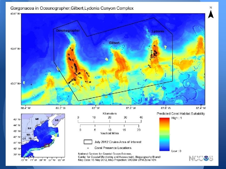
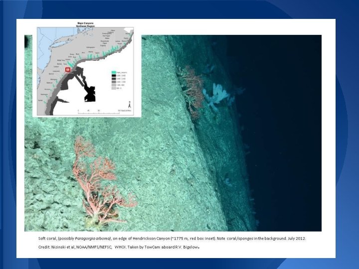
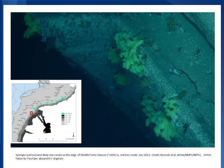
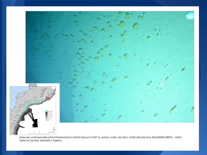
Ground-truthing the Model In July 2012, the NOAA Ship Bigelow visited 3 'hotspots' predicted by the model, and surveyed sites using WHOI’s Tow. Cam. High-resolution multibeam bathymetry collected by NOAA/OAR/OER aboard NOAA Ships Hassler and Okeanos Explorer was used to refine model predictions. WHOI Tow. Cam being deployed aboard the NOAA Ship Bigelow in July, 2012 High-Res Bathy data from OER This cruise was part of the Atlantic Canyons Undersea Mapping Expeditio. Ns (ACUMEN) partnership : http: //oceanexplorer. noaa. gov/okeanos/explorations/acumen 12/summary/welcome. html

Ground-truthing the Model RESULT Model qualitatively validated: all camera tow sites that were observed to be hotspots of coral abundance and diversity were also predicted hotspots of suitability based on the regional model

Future Work • • • Quantitative ground-truthing of the model is underway, including assessment of the prediction skill of the model and correlation between predicted habitat suitability and coral frequency/abundance observations. Georeferenced coral presence/absence and abundance data from July 2012 cruise, along with additional high resolution oceanographic/environmental data, is expected to help improve future iterations of the habitat suitability model Model outputs will be made publicly available via MARCO, BOEM/CSC Multipurpose Marine Cadastre, and other appropriate data portals

ACKNOWLEDGMENTS This work was a joint effort of the NOAA/NMFS Northeast Fisheries Science Center James J. Howard Marine Science Laboratory in Sandy Hook, NJ and the NOAA/NOS National Centers for Coastal Ocean Science in Silver Spring, MD. We are grateful to Tim Battista, Tim Shank, Tom Hourigan, Eric Cordes, Greg Boland, Andrew Davies, John Guinotte and Peter Etnoyer for discussions that contributed to the development of this project. Donna Johnson, Laughlin Siceloff, and Amit Malhotra provided technical assistance. This project was partially supported by funding from the NOAA Deep-Sea Coral Research and Technology Program (DSCRTP), the NOAA Coastal and Marine Spatial Planning Program, and the North Atlantic Regional Team (NART). The July 2012 Deep-Sea Coral Survey/Groundtruthing Cruise was led by Martha Nizinski (NOAA/NMFS/NEFSC National Systematics Laboratory) and brought together partners from NOAA/OAR/OER (Mashkoor Malik) and WHOI (Tim Shank). This cruise was part of the Atlantic Canyons Undersea Mapping Expeditio. Ns (ACUMEN) partnership which brought together several NOAA line offices, other federal agencies, and states: http: //oceanexplorer. noaa. gov/okeanos/explorations/acumen 12/summary/welcome. html

Contact information Modeling Brian Kinlan Marine Spatial Ecologist NOAA National Ocean Service NCCOS-CCMA-Biogeography Branch 1305 East-West Hwy, SSMC-4, N/SCI-1, #9224 Silver Spring, MD 20910 -3281 301 -713 -3028 x 157 Brian. Kinlan@NOAA. gov Cruises/Field Work Martha Nizinski Zoologist NOAA/NMFS/NEFSC National Systematics Laboratory Smithsonian Institution PO Box 37012 NHB, WC-57, MRC-153 Washington, DC 20013 -7012 202 -633 -0671 Nizinski@SI. edu Dave Packer Marine Ecologist Coastal Ecology Branch National Oceanic and Atmospheric Administration National Marine Fisheries Service Northeast Fisheries Science Center James J. Howard Marine Sciences Laboratory Highlands, NJ 08535 732 -872 -3044 Dave. Packer@NOAA. gov
- Slides: 30