Deep Neural Network optimization quantization and finetuning Barry

Deep Neural Network optimization: quantization and fine-tuning Barry de Bruin Electrical Engineering – Electronic Systems group

Outline of Today’s Lecture Main theme: DNN quantization and fine-tuning 1. Introduction 2. Overview 3. Approaches 4. Quantization for a off-the-shelf platforms i. e. an integer-based data path a) Preliminaries b) Quantization methodology c) Fixed-point fine-tuning 5. Conclusion 2

Recap – last lecture Observation: 1 off-chip memory access energy = 1000 s of arithmetic ops. Solution: DNN model compression! ‒ Last lecture: ‒ ‒ model pruning (neurons, filters, kernels, layer) construct simpler filters (e. g. decomposition) ‒ This lecture: Quantization of activations, weights, and even gradients. Quantization techniques are orthogonal/complementary! 3

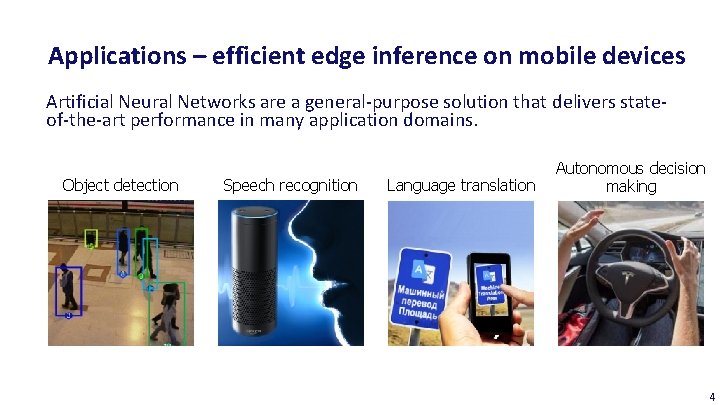
Applications – efficient edge inference on mobile devices Artificial Neural Networks are a general-purpose solution that delivers stateof-the-art performance in many application domains. Object detection Speech recognition Language translation Autonomous decision making 4

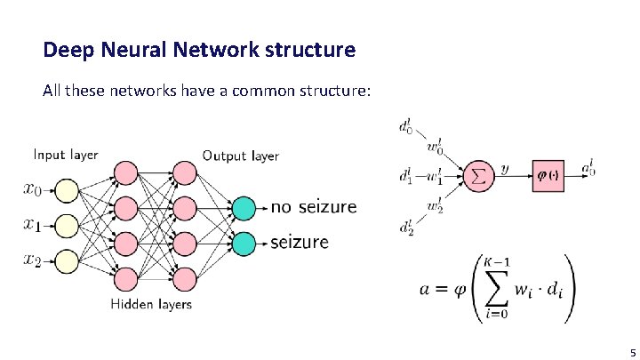
Deep Neural Network structure All these networks have a common structure: 5

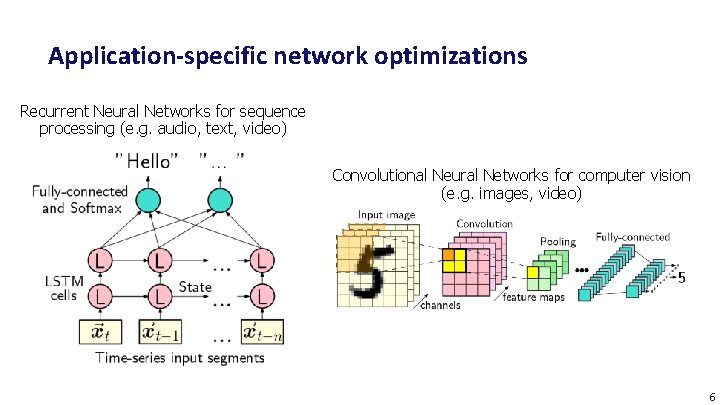
Application-specific network optimizations Recurrent Neural Networks for sequence processing (e. g. audio, text, video) Convolutional Neural Networks for computer vision (e. g. images, video) 6

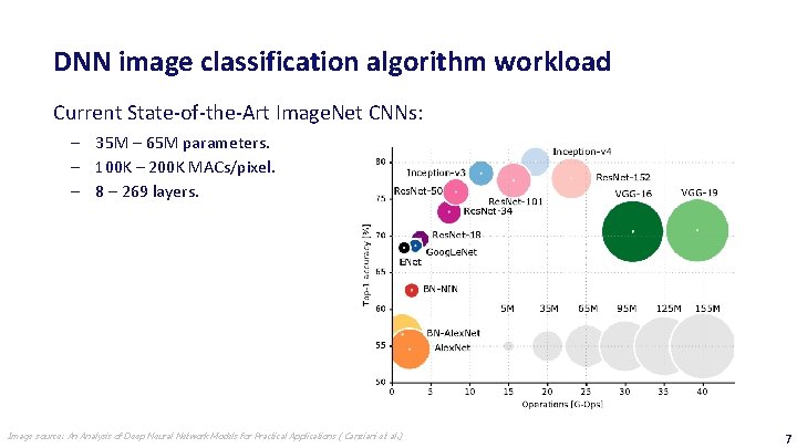
DNN image classification algorithm workload Current State-of-the-Art Image. Net CNNs: ‒ 35 M – 65 M parameters. ‒ 100 K – 200 K MACs/pixel. ‒ 8 – 269 layers. Image source: An Analysis of Deep Neural Network Models for Practical Applications ( Canziani et al. ) 7

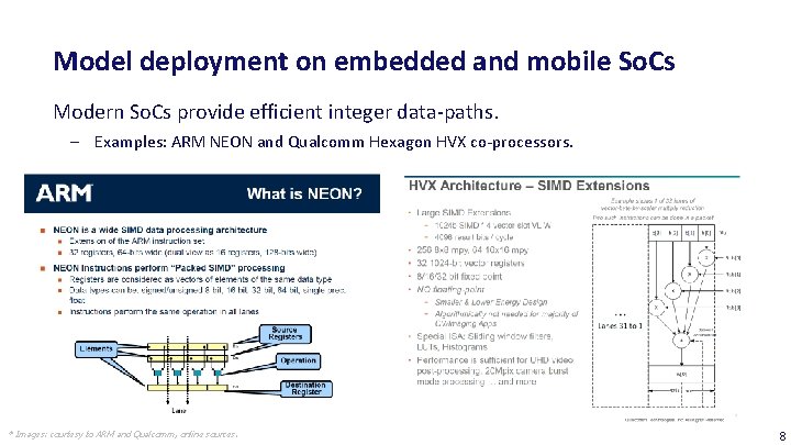
Model deployment on embedded and mobile So. Cs Modern So. Cs provide efficient integer data-paths. ‒ Examples: ARM NEON and Qualcomm Hexagon HVX co-processors. * Images: courtesy to ARM and Qualcomm, online sources. 8

Outline of Today’s Lecture Main theme: DNN quantization and fine-tuning 1. Introduction 2. Overview 3. Approaches 4. Quantization for a off-the-shelf platforms i. e. an integer-based data path a) Preliminaries b) Quantization methodology c) Fixed-point fine-tuning 5. Conclusion 9

What is DNN model quantization? Reduction of the number of bits (i. e. precision) of ‒ weights to reduce model size and weight access cost. ‒ feature maps to reduce intermediate storage and access cost. ‒ gradients to save communication bandwidth in distributed training and enables efficient training on platforms such as FPGAs. ‒ However, learning requires higher precision than inference → best to concentrate on weights and activations! to save energy and/or increase throughput while preserving accuracy! 10

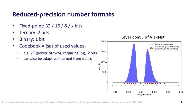
Reduced-precision number formats Layer conv 3 of Alex. Net Image source: Deep Compression: Compressing Deep Neural Networks with Pruning, Trained Quantization and Huffman Coding – S. Han et al. (ICLR 2016) 11

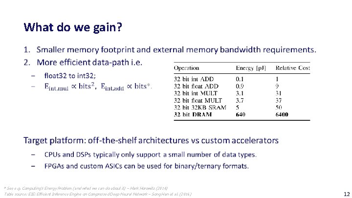
What do we gain? * See e. g. Computing’s Energy Problem (and what we can do about it) – Mark Horowitz (2014) Table source: EIE: Efficient Inference Engine on Compressed Deep Neural Network – Song Han et al. (2016) 12

Outline of Today’s Lecture Main theme: DNN quantization and fine-tuning 1. Introduction 2. Overview 3. Approaches 4. Quantization for a off-the-shelf platforms i. e. an integer-based data path a) Preliminaries b) Quantization methodology c) Fixed-point fine-tuning 5. Conclusion 13

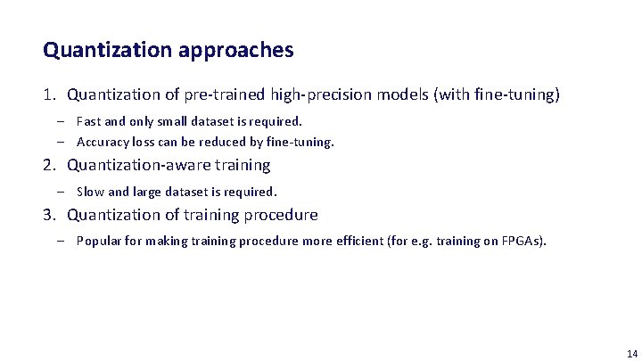
Quantization approaches 1. Quantization of pre-trained high-precision models (with fine-tuning) ‒ Fast and only small dataset is required. ‒ Accuracy loss can be reduced by fine-tuning. 2. Quantization-aware training ‒ Slow and large dataset is required. 3. Quantization of training procedure ‒ Popular for making training procedure more efficient (for e. g. training on FPGAs). 14

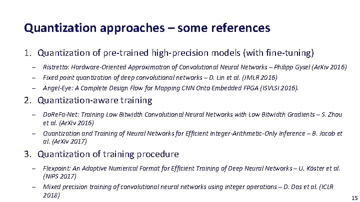
Quantization approaches – some references 1. Quantization of pre-trained high-precision models (with fine-tuning) ‒ ‒ ‒ Ristretto: Hardware-Oriented Approximation of Convolutional Neural Networks – Philipp Gysel (Ar. Xiv 2016) Fixed point quantization of deep convolutional networks – D. Lin et al. (JMLR 2016) Angel-Eye: A Complete Design Flow for Mapping CNN Onto Embedded FPGA (ISVLSI 2016). 2. Quantization-aware training ‒ ‒ Do. Re. Fa-Net: Training Low Bitwidth Convolutional Neural Networks with Low Bitwidth Gradients – S. Zhou et al. (Ar. Xiv 2016) Quantization and Training of Neural Networks for Efficient Integer-Arithmetic-Only Inference – B. Jacob et al. (Ar. Xiv 2017) 3. Quantization of training procedure ‒ ‒ Flexpoint: An Adaptive Numerical Format for Efficient Training of Deep Neural Networks – U. Köster et al. (NIPS 2017) Mixed precision training of convolutional neural networks using integer operations – D. Das et al. (ICLR 2018) 15

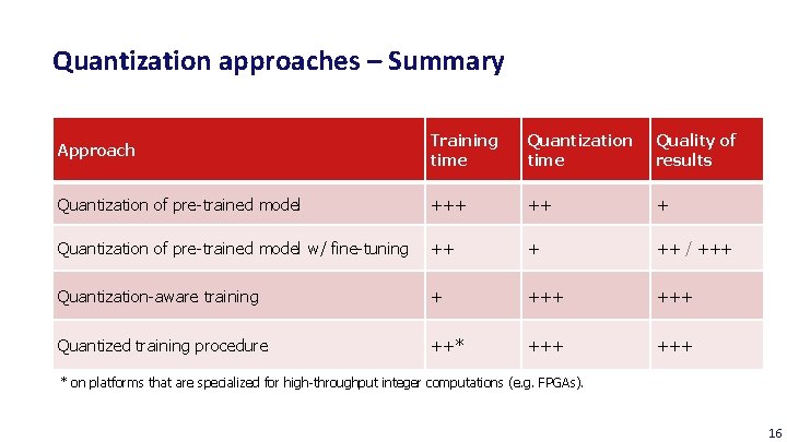
Quantization approaches – Summary Approach Training time Quantization time Quality of results Quantization of pre-trained model +++ ++ + Quantization of pre-trained model w/ fine-tuning ++ + ++ / +++ Quantization-aware training + +++ Quantized training procedure ++* +++ * on platforms that are specialized for high-throughput integer computations (e. g. FPGAs). 16

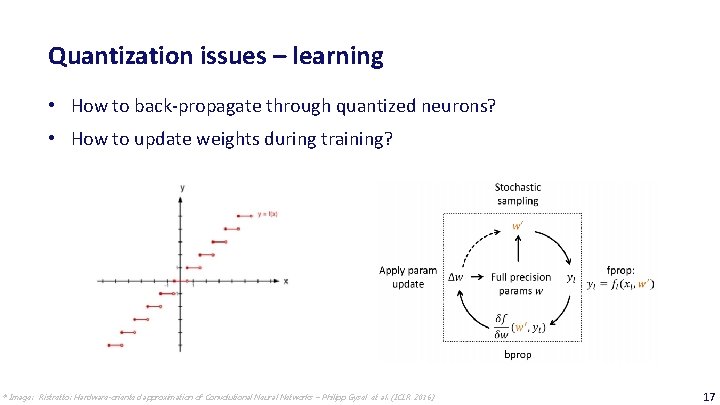
Quantization issues – learning • How to back-propagate through quantized neurons? • How to update weights during training? * Image: Ristretto: Hardware-oriented approximation of Convolutional Neural Networks – Philipp Gysel et al. (ICLR 2016) 17

Quantization issues – finding a good solution • How to quantize a single layer? ‒ How many bits do we use for weights/activations? • How to quantize multiple layers? ‒ Different fixed-point format for every layer? ‒ Brute force solution space or heuristic? 18

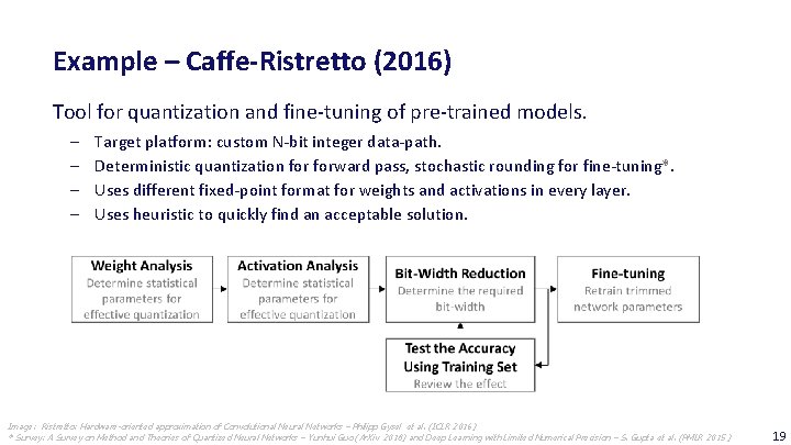
Example – Caffe-Ristretto (2016) Tool for quantization and fine-tuning of pre-trained models. ‒ ‒ Target platform: custom N-bit integer data-path. Deterministic quantization forward pass, stochastic rounding for fine-tuning*. Uses different fixed-point format for weights and activations in every layer. Uses heuristic to quickly find an acceptable solution. Image: Ristretto: Hardware-oriented approximation of Convolutional Neural Networks – Philipp Gysel et al. (ICLR 2016) * Survey: A Survey on Method and Theories of Quantized Neural Networks – Yunhui Guo (Ar. Xiv 2018) and Deep Learning with Limited Numerical Precision – S. Gupta et al. (PMLR 2015 ) 19

Outline of Today’s Lecture Main theme: DNN quantization and fine-tuning 1. Introduction 2. Overview 3. Approaches 4. Quantization for a off-the-shelf platforms i. e. an integer-based data path a) Preliminaries b) Quantization methodology c) Fixed-point fine-tuning 5. Conclusion 20

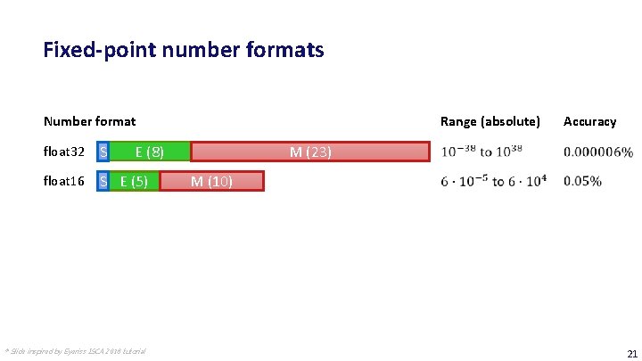
Fixed-point number formats Number format float 32 S float 16 S E (5) int 32 S int 16 S int 8 S Range (absolute) E (8) Accuracy M (23) M (10) M (31) M (15) M (7) * Slide inspired by Eyeriss ISCA 2018 tutorial 21

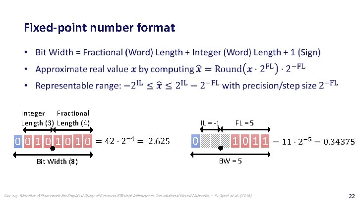
Fixed-point number format Fractional Integer Length (3) Length (4) 00101010 Bit Width (8) IL = -1 0 FL = 5 1011 BW = 5 See e. g. Ristretto: A Framework for Empirical Study of Resource-Efficient Inference in Convolutional Neural Networks – P. Gysel et al. (2018) 22

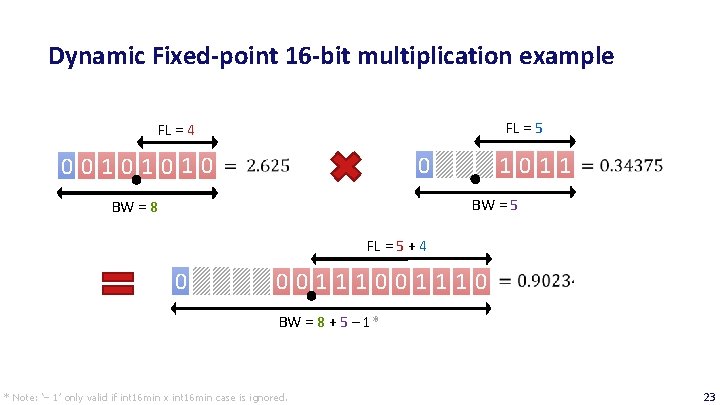
Dynamic Fixed-point 16 -bit multiplication example FL = 5 FL = 4 00101010 1011 0 BW = 5 BW = 8 FL = 5 + 4 0 001110 BW = 8 + 5 – 1* * Note: ‘– 1’ only valid if int 16 min x int 16 min case is ignored. 23

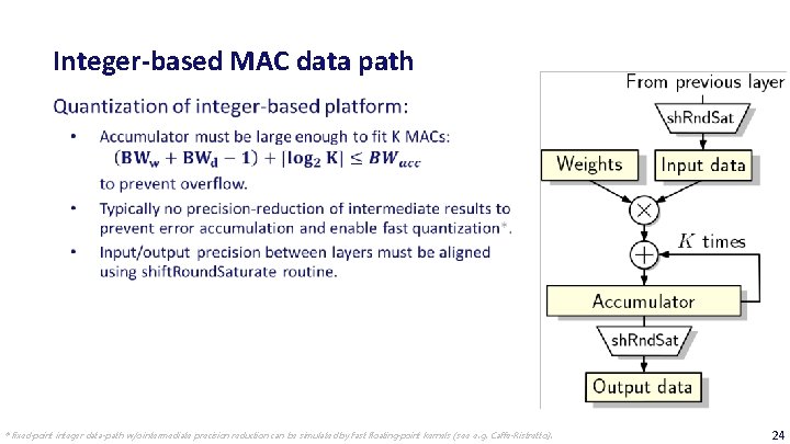
Integer-based MAC data path * fixed-point integer data-path w/o intermediate precision reduction can be simulated by fast floating-point kernels (see e. g. Caffe-Ristretto). 24

Outline of Today’s Lecture Main theme: DNN quantization and fine-tuning 1. Introduction 2. Overview 3. Approaches 4. Quantization for a off-the-shelf platforms i. e. an integer-based data path a) Preliminaries b) Quantization methodology c) Fixed-point fine-tuning 5. Conclusion 25

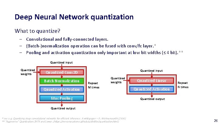
Deep Neural Network quantization What to quantize? ‒ Convolutional and fully-connected layers. ‒ (Batch-)normalization operation can be fused with conv/fc layer. * ‒ Pooling and activation quantization only important at low bit widths (≤ 4 bit). ** Quantized input Quantized weights Quantized input Quantized Conv 2 D Batch Normalization Quantized Activation Repeat M times Quantized weights Max Pooling Quantized Linear Quantized Activation Repeat N times Quantized output * see e. g. Quantizing deep convolutional networks for efficient inference: A whitepaper – R. Krishnamoorthi (2018) ** ”Aggressive” Quantization: INT 4 and Lower. (https: //nervanasystems. github. io/distiller/quantization. html) 26

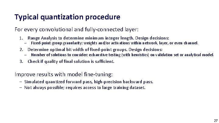
Typical quantization procedure For every convolutional and fully-connected layer: 1. Range Analysis to determine minimum integer length. Design decisions: ‒ Fixed-point group granularity: weights and/or activations within network, layer, or even channel. 2. Determine optimal bit width of fixed-point groups. Design decisions: ‒ Number of solutions to consider: exhaustive testing (with heuristics) on validation set or analytical model. 3. Check if quality of final solution is sufficient. Improve results with model fine-tuning: ‒ Simulated quantized forward pass, high-precision backward pass. ‒ Not always possible; requires access to large training dataset. 27

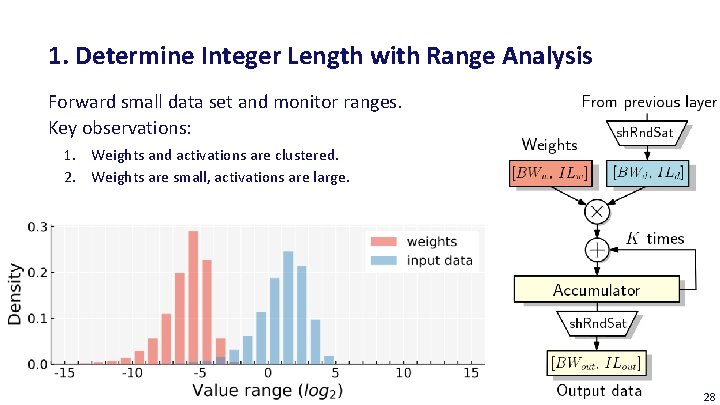
1. Determine Integer Length with Range Analysis Forward small data set and monitor ranges. Key observations: 1. Weights and activations are clustered. 2. Weights are small, activations are large. 28

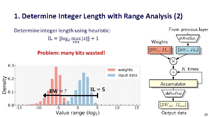
1. Determine Integer Length with Range Analysis (2) 29

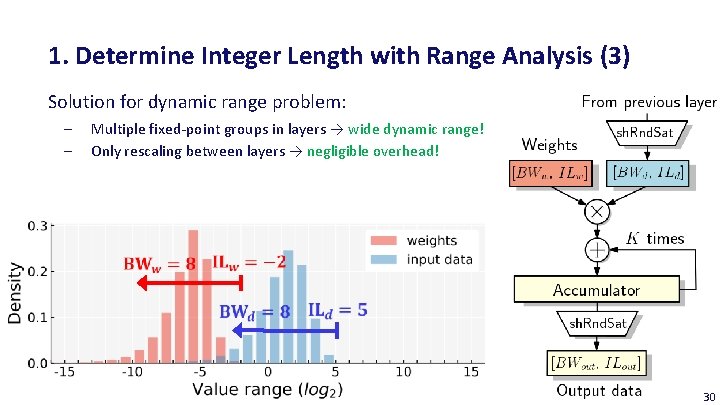
1. Determine Integer Length with Range Analysis (3) Solution for dynamic range problem: ‒ ‒ Multiple fixed-point groups in layers → wide dynamic range! Only rescaling between layers → negligible overhead! 30

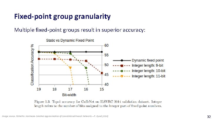
Fixed-point group granularity Multiple fixed-point groups result in superior accuracy: Image source: Ristretto: Hardware-Oriented Approximation of Convolutional Neural Networks – P. Gysel (2016) 32

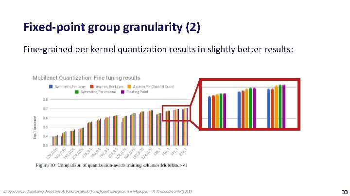
Fixed-point group granularity (2) Fine-grained per kernel quantization results in slightly better results: Image source: Quantizing deep convolutional networks for efficient inference: A whitepaper – R. Krishnamoorthi (2018) 33

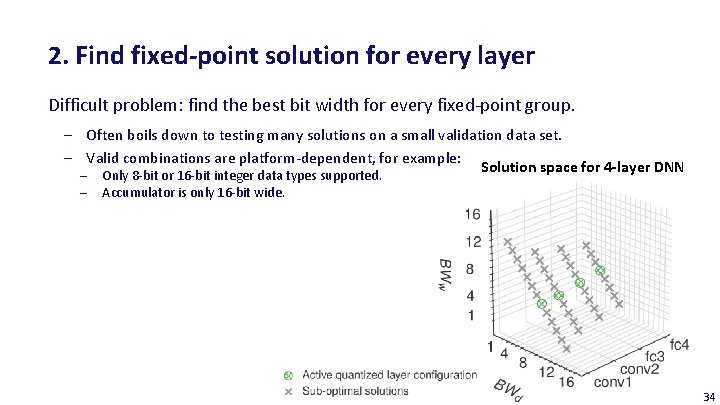
2. Find fixed-point solution for every layer Difficult problem: find the best bit width for every fixed-point group. ‒ Often boils down to testing many solutions on a small validation data set. ‒ Valid combinations are platform-dependent, for example: Solution space for 4 -layer DNN ‒ Only 8 -bit or 16 -bit integer data types supported. ‒ Accumulator is only 16 -bit wide. 34

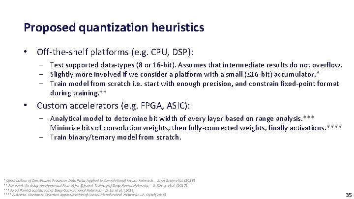
Proposed quantization heuristics • Off-the-shelf platforms (e. g. CPU, DSP): ‒ Test supported data-types (8 or 16 -bit). Assumes that intermediate results do not overflow. ‒ Slightly more involved if we consider a platform with a small (≤ 16 -bit) accumulator. * ‒ Train model from scratch i. e. start with enough precision, and constrain fixed-point format during training. ** • Custom accelerators (e. g. FPGA, ASIC): ‒ Analytical model to determine bit width of every layer based on range analysis. *** ‒ Minimize bits of convolution weights, then fully-connected weights, finally activations. **** ‒ Train binary/ternary model from scratch. * Quantization of Constrained Processor Data Paths Applied to Convolutional Neural Networks – B. de Bruin et al. (2018) ** Flexpoint: An Adaptive Numerical Format for Efficient Training of Deep Neural Networks – U. Köster et al. (2017) *** Fixed Point Quantization of Deep Convolutional Networks – D. Lin et al. (2016) **** Ristretto: Hardware-Oriented Approximation of Convolutional Neural Networks – P. Gysel (2016) 35

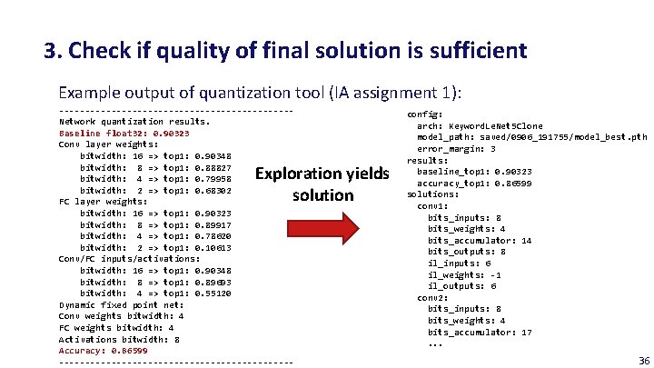
3. Check if quality of final solution is sufficient Example output of quantization tool (IA assignment 1): ----------------------Network quantization results. Baseline float 32: 0. 90323 Conv layer weights: bitwidth: 16 => top 1: 0. 90348 bitwidth: 8 => top 1: 0. 88827 bitwidth: 4 => top 1: 0. 79958 bitwidth: 2 => top 1: 0. 68302 FC layer weights: bitwidth: 16 => top 1: 0. 90323 bitwidth: 8 => top 1: 0. 89917 bitwidth: 4 => top 1: 0. 78620 bitwidth: 2 => top 1: 0. 10613 Conv/FC inputs/activations: bitwidth: 16 => top 1: 0. 90348 bitwidth: 8 => top 1: 0. 89693 bitwidth: 4 => top 1: 0. 55120 Dynamic fixed point net: Conv weights bitwidth: 4 FC weights bitwidth: 4 Activations bitwidth: 8 Accuracy: 0. 86599 ----------------------- Exploration yields solution config: arch: Keyword. Le. Net 5 Clone model_path: saved/0906_191755/model_best. pth error_margin: 3 results: baseline_top 1: 0. 90323 accuracy_top 1: 0. 86599 solutions: conv 1: bits_inputs: 8 bits_weights: 4 bits_accumulator: 14 bits_outputs: 8 il_inputs: 6 il_weights: -1 il_outputs: 6 conv 2: bits_inputs: 8 bits_weights: 4 bits_accumulator: 17. . . 36

Outline of Today’s Lecture Main theme: DNN quantization and fine-tuning 1. Introduction 2. Overview 3. Approaches 4. Quantization for a off-the-shelf platforms i. e. an integer-based data path a) Preliminaries b) Quantization methodology c) Fixed-point fine-tuning 5. Conclusion 37

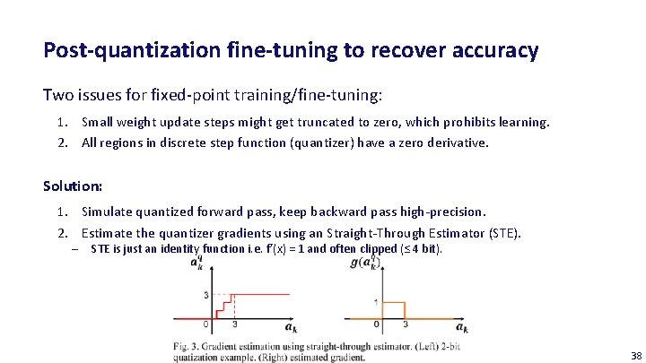
Post-quantization fine-tuning to recover accuracy Two issues for fixed-point training/fine-tuning: 1. Small weight update steps might get truncated to zero, which prohibits learning. 2. All regions in discrete step function (quantizer) have a zero derivative. Solution: 1. Simulate quantized forward pass, keep backward pass high-precision. 2. Estimate the quantizer gradients using an Straight-Through Estimator (STE). ‒ STE is just an identity function i. e. f’(x) = 1 and often clipped (≤ 4 bit). 38

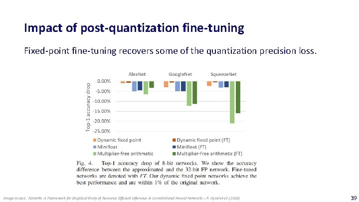
Impact of post-quantization fine-tuning Fixed-point fine-tuning recovers some of the quantization precision loss. Image source: Ristretto: A Framework for Empirical Study of Resource-Efficient Inference in Convolutional Neural Networks – P. Gysel et al. (2018) 39

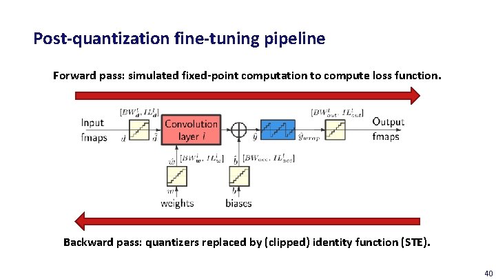
Post-quantization fine-tuning pipeline Forward pass: simulated fixed-point computation to compute loss function. Backward pass: quantizers replaced by (clipped) identity function (STE). 40

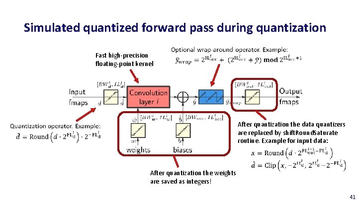
Simulated quantized forward pass during quantization Fast high-precision floating-point kernel After quantization the data quantizers are replaced by shift. Round. Saturate routine. Example for input data: After quantization the weights are saved as integers! 41

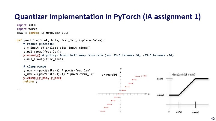
Quantizer implementation in Py. Torch (IA assignment 1) import math import torch pow 2 = lambda x: math. pow(2, x) def quantize(input, bits, frac_len, inplace=False): # reduce precision y = input if inplace else input. clone() y. mul_(pow 2(frac_len)) y. round_() # policy: Round half away from zero (ex: 23. 5 becomes 24, -23. 5 becomes -24) y. mul_(pow 2(-frac_len)) # clamp range y_min = -pow 2(bits-1) * pow 2(-frac_len) y_max = (pow 2(bits-1)-1) * pow 2(-frac_len) y. clamp_(y_min, y_max) return y y = round(x) . . . 42

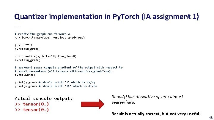
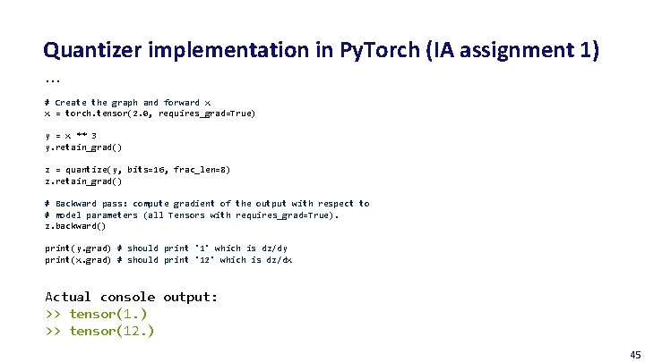
Quantizer implementation in Py. Torch (IA assignment 1). . . # Create the graph and forward x x = torch. tensor(2. 0, requires_grad=True) y = x ** 3 y. retain_grad() z = quantize(y, bits=16, frac_len=8) z. retain_grad() # Backward pass: compute gradient of the output with respect to # model parameters (all Tensors with requires_grad=True). z. backward() print(y. grad) # should print '1' which is dz/dy print(x. grad) # should print '12' which is dz/dx Actual console output: >> tensor(0. ) Round() has derivative of zero almost everywhere. Result is actually correct, but not very useful! 43

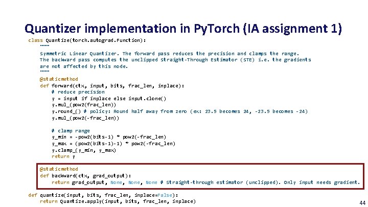
Quantizer implementation in Py. Torch (IA assignment 1) class Quantize(torch. autograd. Function): """ Symmetric Linear Quantizer. The forward pass reduces the precision and clamps the range. The backward pass computes the unclipped Straight-Through Estimator (STE) i. e. the gradients are not affected by this node. """ @staticmethod def forward(ctx, input, bits, frac_len, inplace): # reduce precision y = input if inplace else input. clone() y. mul_(pow 2(frac_len)) y. round_() # policy: Round half away from zero (ex: 23. 5 becomes 24, -23. 5 becomes -24) y. mul_(pow 2(-frac_len)) # clamp range y_min = -pow 2(bits-1) * pow 2(-frac_len) y_max = (pow 2(bits-1)-1) * pow 2(-frac_len) y. clamp_(y_min, y_max) return y @staticmethod def backward(ctx, grad_output): return grad_output, None, None # Straight-through estimator (unclipped). Only input needs gradient. def quantize(input, bits, frac_len, inplace=False): return Quantize. apply(input, bits, frac_len, inplace) 44

Quantizer implementation in Py. Torch (IA assignment 1). . . # Create the graph and forward x x = torch. tensor(2. 0, requires_grad=True) y = x ** 3 y. retain_grad() z = quantize(y, bits=16, frac_len=8) z. retain_grad() # Backward pass: compute gradient of the output with respect to # model parameters (all Tensors with requires_grad=True). z. backward() print(y. grad) # should print '1' which is dz/dy print(x. grad) # should print '12' which is dz/dx Actual console output: >> tensor(1. ) >> tensor(12. ) 45

Outline of Today’s Lecture Main theme: DNN quantization and fine-tuning 1. Introduction 2. Overview 3. Approaches 4. Quantization for a off-the-shelf platforms i. e. an integer-based data path a) Preliminaries b) Quantization methodology c) Fixed-point fine-tuning 5. Conclusion 46

Summary – quantization for off-the-shelf platforms • For efficient deployment on embedded or mobile devices models are converted to integer-only arithmetic. We can either convert a pre-trained model to reduced-precision, or train a quantized model from scratch. • A symmetric linear quantizer is a conventional fixed-point format. Asymmetric linear quantizers are used if the value distribution is not symmetric. Non-linear quantizers are sometimes used in the literature, but difficult to efficiently use on general-purpose platforms. • Multiple fixed-point groups are used to capture the different distributions within layers of the network more efficiently. • Typically, a number of quantization solutions will be tested, depending on the platform characteristics (supported data types and accumulator size). • Model fine-tuning or retraining is essential to recover some of the lost accuracy. Some measures needs to be taken to enable simulated quantized fine-tuning. 47

Conclusions • Quantization are an essential tool for efficient model deployment. • These techniques can be combined with other compression methods, such as pruning. • 8 -bit data and weights with 32 -bit accumulators is sufficient for recent DNNs. Next Up: Binary Neural Networks • For custom accelerators there is a huge shift from fixed-point to binary/ternary networks, which can potentially replace MACs by XNOR and POPCOUNT instructions. • Next lecture we will investigate the training and deployment of a Binary Neural Network. 48

Deep Neural Network optimization: quantization and fine-tuning Barry de Bruin Electrical Engineering – Electronic Systems group