Deep Learning Species Distribution Modelling Piotr Usewicz 2019
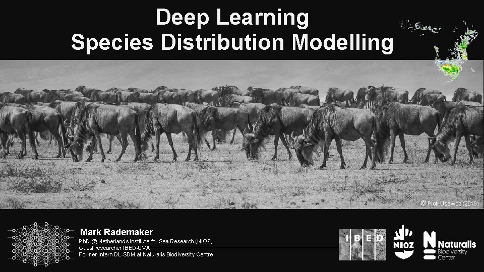
Deep Learning Species Distribution Modelling © Piotr Usewicz (2019) Mark Rademaker Ph. D @ Netherlands Institute for Sea Research (NIOZ) Guest researcher IBED-UVA Former Intern DL-SDM at Naturalis Biodiversity Centre
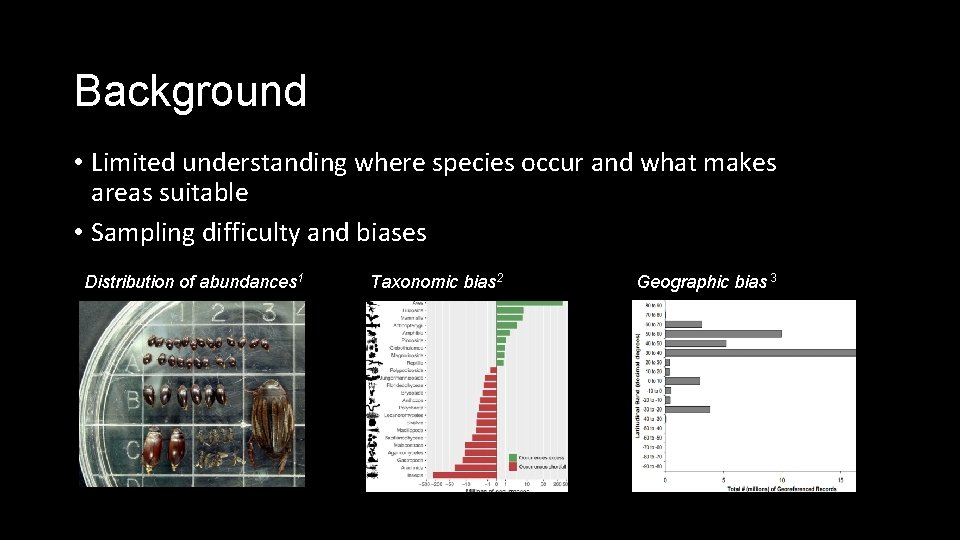
Background • Limited understanding where species occur and what makes areas suitable • Sampling difficulty and biases Distribution of abundances 1 Taxonomic bias 2 Geographic bias 3
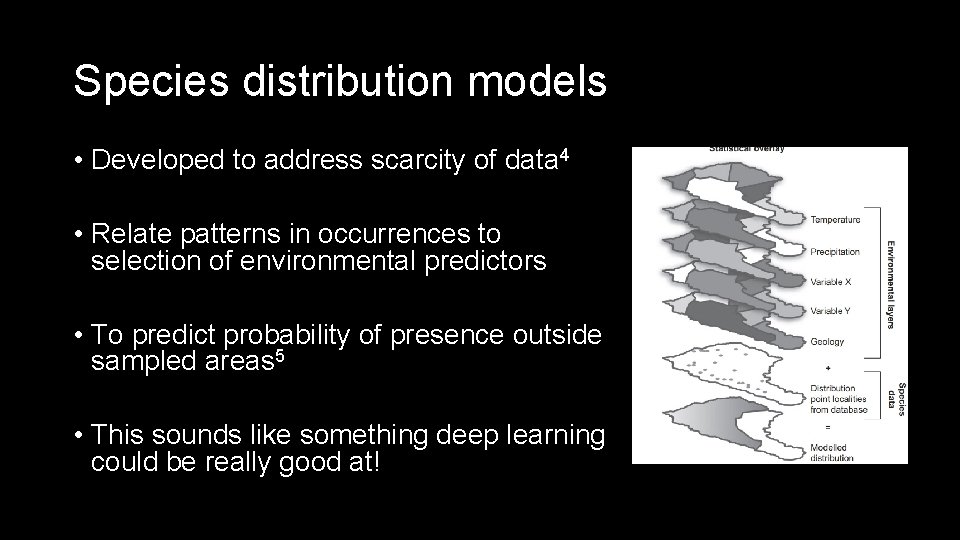
Species distribution models • Developed to address scarcity of data 4 • Relate patterns in occurrences to selection of environmental predictors • To predict probability of presence outside sampled areas 5 • This sounds like something deep learning could be really good at!
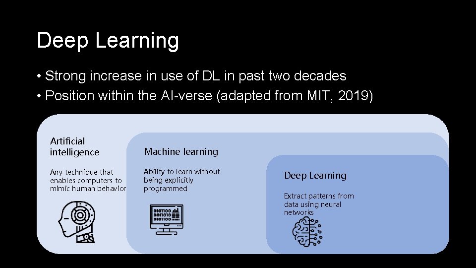
Deep Learning • Strong increase in use of DL in past two decades • Position within the AI-verse (adapted from MIT, 2019) Artificial intelligence Machine learning Any technique that enables computers to mimic human behavior Ability to learn without being explicitly programmed Deep Learning Extract patterns from data using neural networks
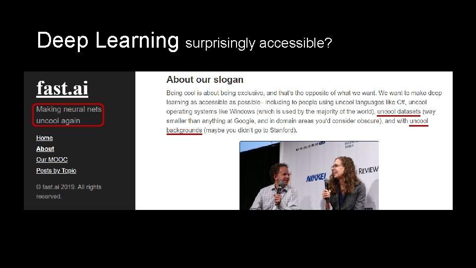
Deep Learning surprisingly accessible?
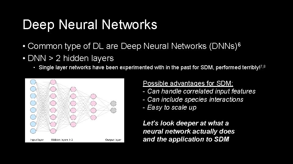
Deep Neural Networks • Common type of DL are Deep Neural Networks (DNNs)6 • DNN > 2 hidden layers • Single layer networks have been experimented with in the past for SDM, performed terribly!7, 8 Possible advantages for SDM: - Can handle correlated input features - Can include species interactions - Easy to scale up Let’s look deeper at what a neural network actually does and the application to SDM
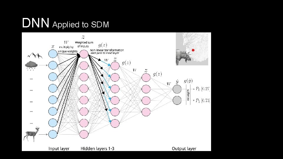
DNN Applied to SDM
The research Aim: • Proof of concept DL-SDM • Using pre-existing dataset of Worlds Ungulates Goals to assess: • Types of input data • Evaluation methods • Model architecture • Performance compared to Max. Ent • Potential for large scale implementation v 3. 6
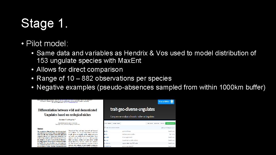
Stage 1. • Pilot model: • Same data and variables as Hendrix & Vos used to model distribution of 153 ungulate species with Max. Ent • Allows for direct comparison • Range of 10 – 882 observations per species • Negative examples (pseudo-absences sampled from within 1000 km buffer)

Stage 1. • Pilot model & performance Comparison to Max. Ent • Performs considerably worse if all species taken into account • Already pretty close if only species >100 occurrences taken into account • What does this mean in terms of predicted global distributions?
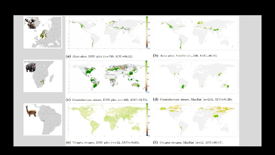
Stage 1. • Pilot model & performance Comparison to Max. Ent • Performs considerably worse if all species taken into account • Already pretty close if only species >100 occurrences taken into account • What does this mean in terms of predicted global distributions?
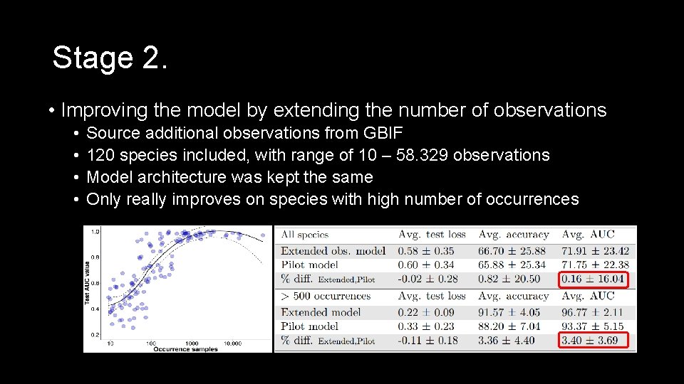
Stage 2. • Improving the model by extending the number of observations • • Source additional observations from GBIF 120 species included, with range of 10 – 58. 329 observations Model architecture was kept the same Only really improves on species with high number of occurrences
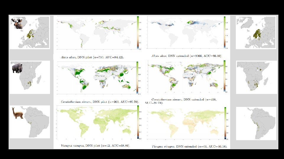
Stage 2. • Improving the model by extending the number of observations • • Source additional observations from GBIF 120 species included, with range of 10 – 58. 329 observations Model architecture was kept the same Only really improves on species with high number of occurrences
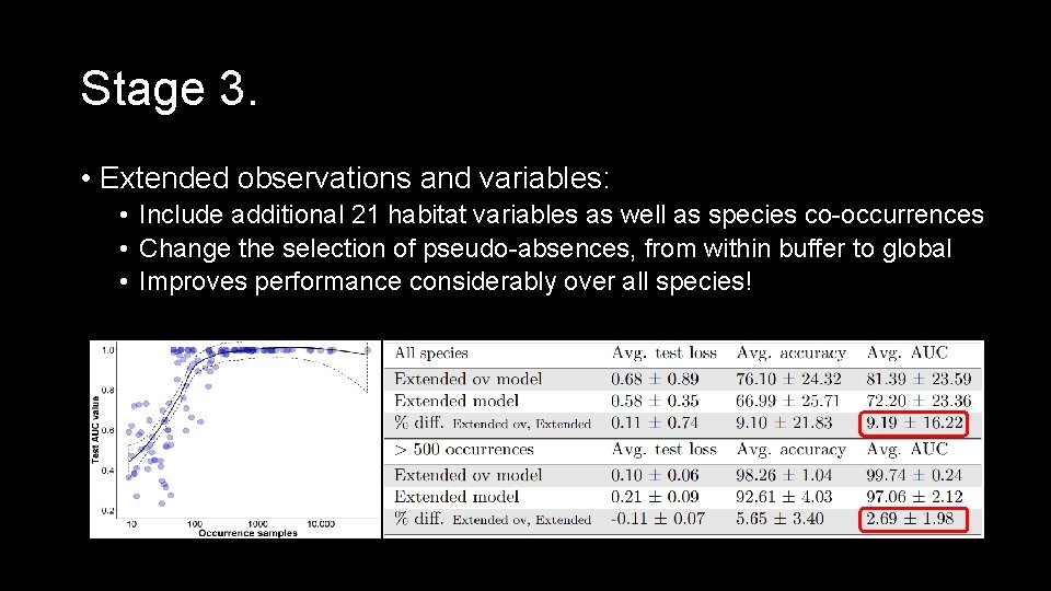
Stage 3. • Extended observations and variables: • Include additional 21 habitat variables as well as species co-occurrences • Change the selection of pseudo-absences, from within buffer to global • Improves performance considerably over all species!
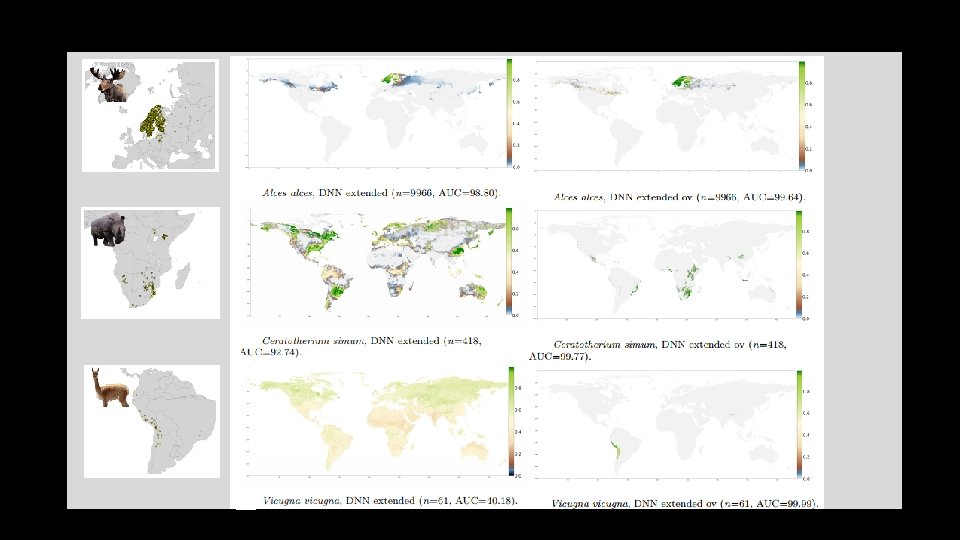
Stage 3. • Extended observations and variables: • Include additional 21 habitat variables as well as species co-occurrences • Change the selection of background locations, from within IUNC Range to entire globe
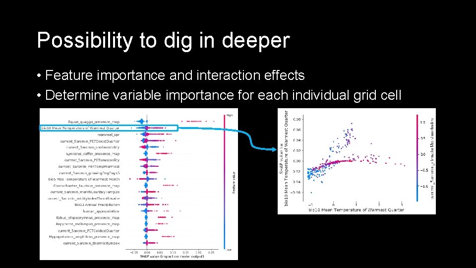
Possibility to dig in deeper • Feature importance and interaction effects • Determine variable importance for each individual grid cell
Relay to research goals • Assess types of input data • Requires both abiotic and biotic environmental variables • Assess model architecture • Relatively shallow with only 4 hidden layers • Evaluation methods • AUC values and prediction maps can be used to evaluate performance and compare with other methods • Performance compared to Max. Ent • Worse for low and similar for large sample size given only abiotic environmental variables • Extending observations, adding (biotic) variable and adjusting pseudo-absence sampling leads to large improvement • Potential for large scale implementation • Not assessed yet, challenge for the future
Future research • From separate model per species to single large multiclassification • • Single model predicting probabilities of presence for all species Likely needs to be much deeper Does not need to learn weights from scratch Can retrain weights to optimize for specific species of interest • Modelling shifting distributions (climate change) • Infuse time-dynamics with species interactions • Would require completely different type of DL-SDM, based on RNN • Comparison with mechanistic theoretical models • Does the DL model find patterns in observational data that validate theory?
Getting started • Free courses • And website • Handy instructional books

Thank you for your attention! • Questions?
References 1. 2. 3. 4. 5. 6. 7. 8. Mc. Gill, B. J. , Etienne, R. S. , Gray, J. S. , Alonso, D. , Anderson, M. J. , Benecha, H. K. , . . . & Hurlbert, A. H. (2007). Species abundance distributions: moving beyond single prediction theories to integration within an ecological framework. Ecology letters, 10(10), 995 -1015. Troudet, J. , et al. “Taxonomic bias in biodiversity data and societal preferences”. In: Scientific Reports, 7(1) (2017), 9132. Collen, B. , et al. “The tropical biodiversity data gap: addressing disparity in global monitoring”. In: Tropical Conservation Science, 1(2) (2008), 75 -88. Antoine Guisan and Niklaus E Zimmermann. “Predictive habitat distribution models in ecology”. In: Ecological modelling, 135. 2 -3 (2000), pp. 147– 186 Cebon, Peter. 1998. Views from the Alps: regional perspectives on climate change. Cambridge, Mass: MIT Press. Yoav Shoham et al. The AI Index 2018 Annual Report. 2018 Shinji Fukuda et al. “Habitat prediction and knowledge extraction for spawning European grayling (Thymallus thymallus L. ) using a broad range of species distribution models”. In: Environmental modelling & software 47 (2013), pp. 1– 6. Xinhai Li and Yuan Wang. “Applying various algorithms for species distribution modelling”. In: Integrative Zoology 8. 2 (2013), pp. 124– 135.
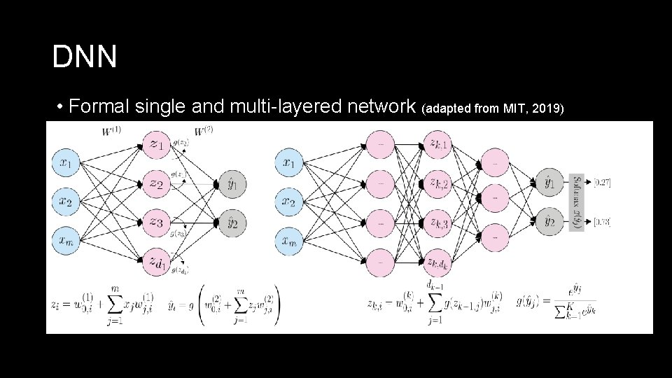
DNN • Formal single and multi-layered network (adapted from MIT, 2019)
- Slides: 22