Deep Learning for DualEnergy XRay Computed Tomography He

- Slides: 1

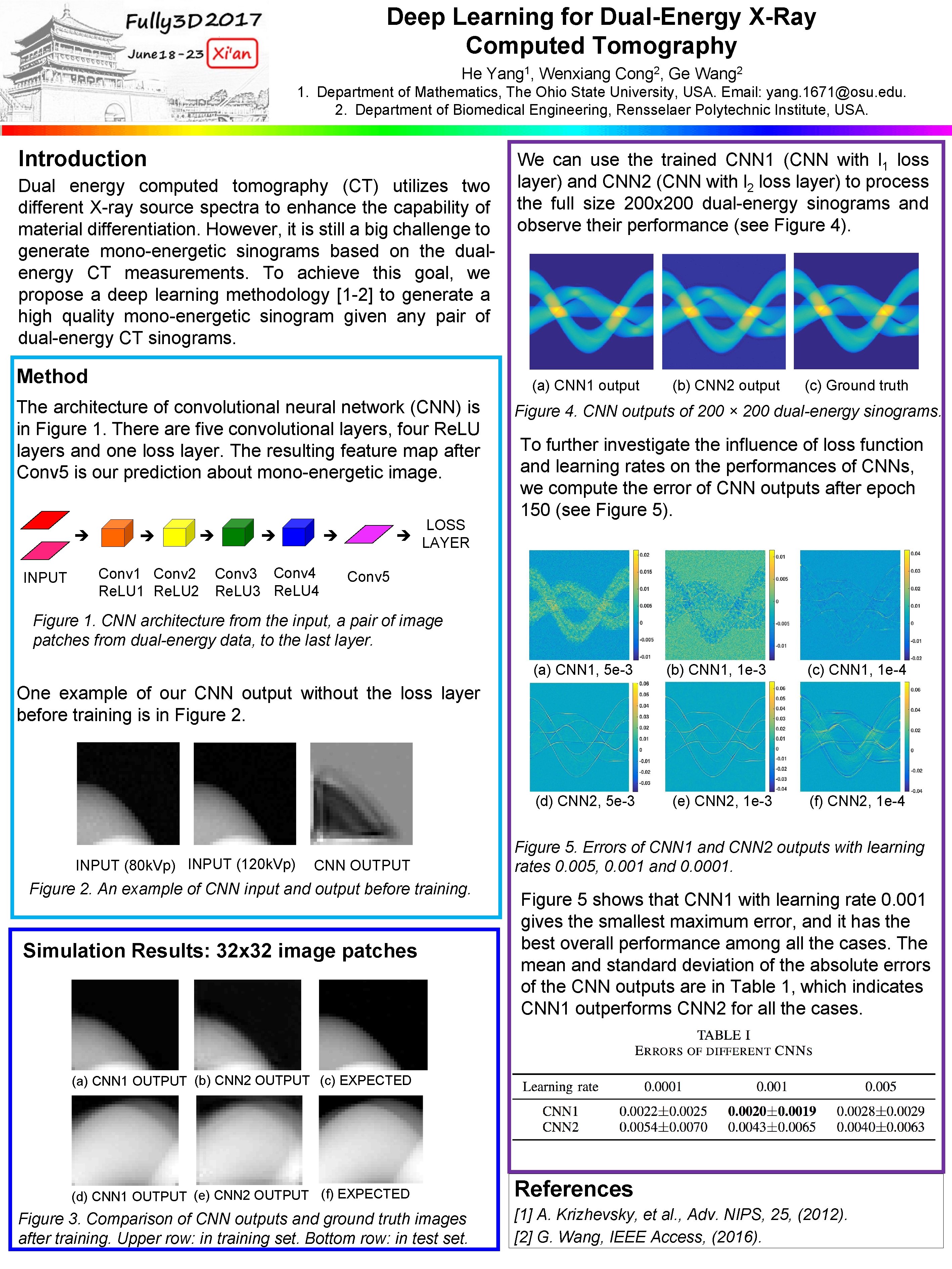
Deep Learning for Dual-Energy X-Ray Computed Tomography He Yang 1, Wenxiang Cong 2, Ge Wang 2 1. Department of Mathematics, The Ohio State University, USA. Email: yang. 1671@osu. edu. 2. Department of Biomedical Engineering, Rensselaer Polytechnic Institute, USA. Introduction Dual energy computed tomography (CT) utilizes two different X-ray source spectra to enhance the capability of material differentiation. However, it is still a big challenge to generate mono-energetic sinograms based on the dualenergy CT measurements. To achieve this goal, we propose a deep learning methodology [1 -2] to generate a high quality mono-energetic sinogram given any pair of dual-energy CT sinograms. Method (a) CNN 1 output The architecture of convolutional neural network (CNN) is in Figure 1. There are five convolutional layers, four Re. LU layers and one loss layer. The resulting feature map after Conv 5 is our prediction about mono-energetic image. INPUT We can use the trained CNN 1 (CNN with l 1 loss layer) and CNN 2 (CNN with l 2 loss layer) to process the full size 200 x 200 dual-energy sinograms and observe their performance (see Figure 4). Conv 1 Conv 2 Re. LU 1 Re. LU 2 LOSS LAYER Conv 3 Conv 4 Re. LU 3 Re. LU 4 (b) CNN 2 output (c) Ground truth Figure 4. CNN outputs of 200 × 200 dual-energy sinograms. To further investigate the influence of loss function and learning rates on the performances of CNNs, we compute the error of CNN outputs after epoch 150 (see Figure 5). Conv 5 Figure 1. CNN architecture from the input, a pair of image patches from dual-energy data, to the last layer. (a) CNN 1, 5 e-3 (b) CNN 1, 1 e-3 (c) CNN 1, 1 e-4 One example of our CNN output without the loss layer before training is in Figure 2. (d) CNN 2, 5 e-3 INPUT (80 k. Vp) INPUT (120 k. Vp) CNN OUTPUT Figure 2. An example of CNN input and output before training. Simulation Results: 32 x 32 image patches (e) CNN 2, 1 e-3 (f) CNN 2, 1 e-4 Figure 5. Errors of CNN 1 and CNN 2 outputs with learning rates 0. 005, 0. 001 and 0. 0001. Figure 5 shows that CNN 1 with learning rate 0. 001 gives the smallest maximum error, and it has the best overall performance among all the cases. The mean and standard deviation of the absolute errors of the CNN outputs are in Table 1, which indicates CNN 1 outperforms CNN 2 for all the cases. (a) CNN 1 OUTPUT (b) CNN 2 OUTPUT (c) EXPECTED (d) CNN 1 OUTPUT (e) CNN 2 OUTPUT (f) EXPECTED Figure 3. Comparison of CNN outputs and ground truth images after training. Upper row: in training set. Bottom row: in test set. References [1] A. Krizhevsky, et al. , Adv. NIPS, 25, (2012). [2] G. Wang, IEEE Access, (2016).