Deep Learning and Convolutional Neural Nets Matt Boutell

Deep Learning and Convolutional Neural Nets Matt Boutell boutell@rose-hulman. edu Image Credit: https: //www. mathworks. com/discovery/convolutional-neural-network. html

Humanengineered feature extraction 384 x 256 x 3 Grid-based Color moments feature vector Background: we are detecting sunsets using the classical image recognition paradigm Classifier (1 hidden Class [-1, 1] layer) Support vector 7 x 7 x 6 machine =294 1. Build model (choose kernel, C) 2. Train (quadratic programming optimization with Lagrange multipliers bounded by Box. Constraints) 3. Predict the class of a new vector by taking the weighted sum of functions of the distances of the vector to the support vectors

Reminder: Basic neural network architecture “Shallow” net Width Each neuron pi = f(x) Or a layer is p = f(x) Depth http: //tx. shu. edu. tw/~purplewoo/Literature/!Data. Analysis/three%20 activation%20 functions. files/NN 1. gif

Humanengineered feature extraction 384 x 256 x 3 Grid-based Color moments feature vector Background: We could swap out the SVM for a traditional (shallow) neural network Classifier (1 -3 layers) Class (0 -1) 7 x 7 x 6 =294 Neural net 4. But the choice of features we extracted may limit accuracy 1. Build model (1 -2 fully-connected hidden network layers) 2. Train (backpropagation to minimize loss) 3. Predict the class of a new vector by extracting features and forward-propagating the features through the neural network

Deep learning is a vague term “Deep” networks typically have 10+ layers. For example, 25, 144, or 177 (we’ll use some of these!) That’s many weights to learn. And more choices of architectures. Should layers be fully connected? How to train them fast enough? Fig: https: //www. slideshare. net/Geeks_Lab/aibigdata-lab-2016 -transfer-learning

Deep learning is a new paradigm in machine learning Deep networks learn both which features to use and how to classify them. There are millions of parameters https: //www. mathworks. com/discovery/convolutional-neural-network. html

Deep learning is an old idea that is now practical In 2012, a deep network was used to win the Image. Net Large Scale Visual Recognition Challenge (14 M annotated images), bringing the top 5 error rate down from the previous 26. 1% to 15. 3%. Deep networks keep winning and improving each year. Why? Faster hardware (GPUs) Access to more training data (www) Algorithmic advances www. deeplearningbook. org/ Olga Russakovsky*, Jia Deng*, Hao Su, Jonathan Krause, Sanjeev Satheesh, Sean Ma, Zhiheng Huang, Andrej Karpathy, Aditya Khosla, Michael Bernstein, Alexander C. Berg and Li Fei-Fei. Image. Net Large Scale Visual Recognition Challenge. IJCV, 2015.

Image classification network layers come in several types Convolution, Re. LU, Pooling https: //www. mathworks. com/discovery/convolutional-neural-network. html

Image classification network layers come in several types Convolution of filters with input. AJ Piergiovanni, CSSE 463 Guest Lecture https: //docs. google. com/presentation/d/15 Lm 6_LTt. Wn. Wp 1 HRPQ 6 lo. I 3 v. N 55 EKNOUi 8 h. OSUyps. Fw 8/

Image classification network layers come in several types Convolution of filters with input

Image classification network layers come in several types Convolution of filters with input. A set of 3 x 3 weights must be learned for each filter. But the same 3 x 3 filter connects every 3 x 3 patch in the first layer with every corresponding neuron in the next. We usually have 10+ such filters per level.

Convolutional layers learn familiar features The first layer filters learn edges and opponent colors, Higher level filters learn more complex features Example Filters Kunihiko Fukushima, “Neocognitron: A self-organizing neural network model for a mechanism of pattern recognition unaffected by shift in position” 2

Image classification network layers come in several types Without nonlinearity, layers collapse. Re. LU (rectified linear unit, blue “Rectifier” in the figure) is one of the simplest non-linear transfer functions. This is transfer function #3: Simple (fast). What is derivative? Can you re-write using max? g(x) = max(______, ______) CC 0, https: //en. wikipedia. org/w/index. php? curid=48817276

Image classification network layers come in several types Because we learn multiple filters at each level, the dimensionality would continue to increase. The solution is to pool data at each layer and downsample. Types: 1. Max-pooling 2. Average-pooling 3. Subsampling only https: //commons. wikimedia. org/wiki/File: Max_pooling. png#filelinks Example of max-pooling.

Q 7 -8 Putting it all together Convolution, Re. LU, Pooling https: //www. mathworks. com/discovery/convolutional-neural-network. html

Gradient Descent ● Goal is to find the min or max of a function ● In calculus, solve f’(x) = 0 ● What if f’(x) can’t be solved for x? ○ Start at some point x, where f’(x) exists Next slides from AJ Piergiovanni, CSSE 463 Guest Lecture https: //docs. google. com/presentation/d/15 Lm 6_LTt. Wn. Wp 1 HRPQ 6 lo. I 3 v. N 55 EKNOUi 8 h. OSUyps. Fw 8/

Gradient Descent

Gradient Descent 5

Gradient Descent - Local Min

Putting it all together Convolution, Re. LU, Pooling 1. Build model (many layers) 2. Train (gradient descent to minimize error function) 3. Predict the class of a new vector by forward propagation through the network https: //www. mathworks. com/discovery/convolutional-neural-network. html

Stochastic Gradient Descent Gradient descent uses all the training data before finding the next location. Stochastic gradient descent divides the training data into mini-batches, which are smaller than the whole data set ○ Trains faster ○ Often converges much faster ○ But may not reach as optimal location as gradient descent So 1 epoch (1 pass through the data set) is made of many mini-batches.

Training a neural network Inputs: 1. the training set (set of images) 2. the network architecture (an array of layers) 3. the options that include hyper-parameters: options = training. Options( 'sgdm', . . . 'Mini. Batch. Size', 32, . . . 'Max. Epochs', 4, . . . 'Initial. Learn. Rate ', 1 e-4, . . . 'Verbose. Frequency', 1, . . . 'Plots', 'training-progress', . . . 'Validation. Data', validate. Images, . . . 'Validation. Frequency', num. Iterations. Per. Epoch); Output: a trained network (with learned weights)

Training a neural network Why do we need 3 sets of data? We know about training and test sets; what is the validation set used for? Hyper-parameters! Train Validation Test

Note: CNNs can classify 1 D signals, like chromatograms, as well. 0. 00 Hi No-peak 0. 17 No-peak 0. 83 Small-peak 0. 00 Peak Each box is a matrix of weights or intermediate values (of neurons)

Note: CNNs can classify 1 D signals, like chromatograms, as well. 768 100 x 16 30 50 x 16 4 25 x 32 12 x 64 0. 00 Hi No-peak 0. 17 No-peak 0. 83 Small-peak 0. 00 Peak Softmax Convolution: learn (3 x 1) filters x 16, Re. LU (nonlinear) Max-pool Conv (3 x 16)x 32, Re. LU, MP Conv (3 x 32)x 64, Re. LU, MP Extract Features Flatten Fullyconnected Classify Boutell and Julian, MSACL 2019

Limitations Deep learning is a black box - the learned weights are often not intuitive They require LOTS of training data. Need many, many (millions) images to get good accuracy when training from scratch

Overcoming limitations: transfer learning Some researchers have released their trained networks. Alex. Net, Google. Net, Res. Net-x, or VGG-19. Why would we do this? # images, speed, accuracy. 1. Can you use them directly? 2. Transfer: Can you swap out and re-train the classification layers for your problem? 3. Can you run the feature extraction part only and save the activations for an SVM to classify? 4. Or do you need to start from scratch? These options are the basis for the next lab and the sunset detector MATLAB docs

Questions?

Visualizing CNNs This next section is the senior thesis work of AJ Piergiovanni, RHIT CS/MA (2015), now studying deep learning at Indiana University. Alternative: new results presented in Stanford course. AJ Piergiovanni, CSSE 463 Guest Lecture https: //docs. google. com/presentation/d/15 Lm 6_LTt. Wn. Wp 1 HRPQ 6 lo. I 3 v. N 55 EKNOUi 8 h. OSUyps. Fw 8/

Deconvolutional neural network Deconvolutional Network Layer Above Reconstruction Convolutional Network Pooled Maps switches Remove Bias and Unpool Pooling, rectification and bias Deconvolve Convolution Reconstruction Layer Below Pooled Maps Source code

Inverting max-pooling ● To invert max-pooling, switches are used to store where the max value is from ○ Some data is lost, but this preserves the max values, which are what affected the feature in the higher levels Zeiler, M. D. & Fergus, R. Visualizing and Understanding Convolutional Networks.

Convolution ● Takes the output from the convolution and convolves it with the transpose of the filters to reconstruct the input Input Convolve with each filter Two outputs One reconstructed output Convolve with transposed filters CNN Deconvolutional Network

t-SNE ● T-distributed Stochastic neighbor embedding (Wikipedia) ● Unsupervised dimensionality reduction technique ● Minimizes the difference between probability distributions ● Maps high dimensional data to 2 D space by preserving the density of the points L. J. P. van der Maaten and G. E. Hinton. Visualizing High-Dimensional Data Using t-SNE.

t-SNE

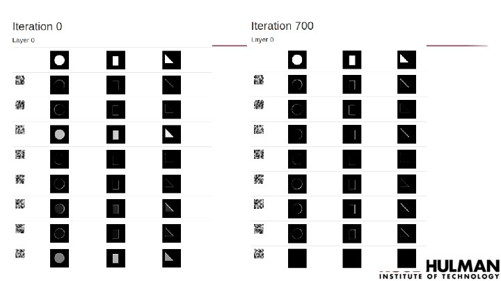
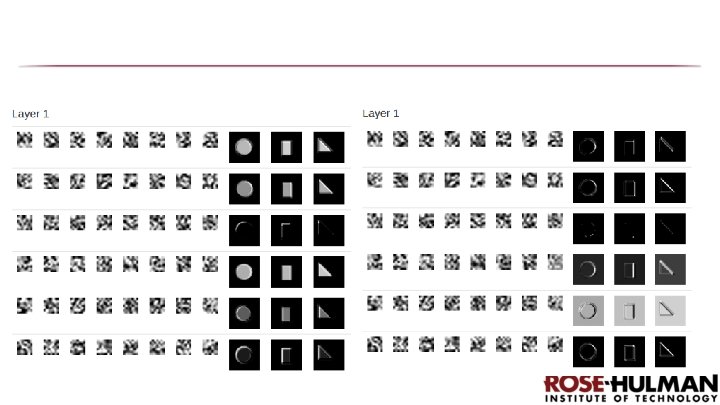
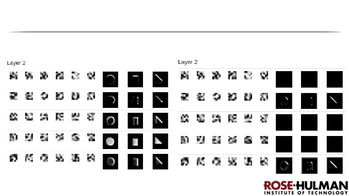
3 -shape classification Trained a CNN to classify images of rectangles, circles and triangles.

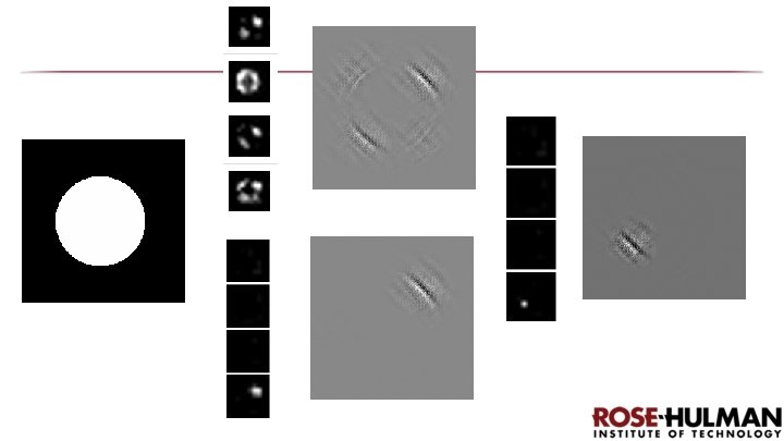
Reconstructed Inputs:

More deconvolution

Title Text