Deep Learning 2 outline NN Basic Autoencoder VAE

Deep Learning 2

outline ● NN Basic ● Autoencoder ● VAE

Programming paradigm

Hierarchy ● Neuron ● Neural networks ● Model ○ CNN, …… ● Framework ○ ○ tensorflow, py. Torch, caffe 2 Keras ● Tool ○ Nvidia digits, Google Auto. ML

Basic 政治大學應用數學系《數學軟體應用》課程的上課筆記 http: //nbviewer. jupyter. org/github/yenlung/nccu-jupyter-math/tree/master/ https: //github. com/fchollet/deep-learning-with-python-notebooks 李宏毅 / 一天搞懂深度學習

MNIST from keras. datasets import mnist (train_images, train_labels), (test_images, test_labels) = mnist. load_data() train_images = train_images. reshape((60000, 28 * 28)) train_images = train_images. astype('float 32') / 255 test_images = test_images. reshape((10000, 28 * 28)) test_images = test_images. astype('float 32') / 255 from keras. utils import to_categorical train_labels = to_categorical(train_labels) test_labels = to_categorical(test_labels)

from keras import models from keras import layers network = models. Sequential() network. add(layers. Dense(512, activation='relu', input_shape=(28 * 28, ))) network. add(layers. Dense(10, activation='softmax')) network. compile(optimizer='rmsprop', loss='categorical_crossentropy', metrics=['accuracy']) network. fit(train_images, train_labels, epochs=5, batch_size=128) test_loss, test_acc = network. evaluate(test_images, test_labels)

autoencoder

autoencoder 1) Autoencoders are data-specific 2) Autoencoders are lossy 3) Autoencoders are learned automatically from data examples

● data denoising ● dimensionality reduction for data visualization

from keras. layers import Input, Dense from keras. models import Model # this is the size of our encoded representations encoding_dim = 32 # 32 floats -> compression of factor 24. 5, assuming the input is 784 floats # this is our input placeholder input_img = Input(shape=(784, )) # "encoded" is the encoded representation of the input encoded = Dense(encoding_dim, activation='relu')(input_img) # "decoded" is the lossy reconstruction of the input decoded = Dense(784, activation='sigmoid')(encoded) # this model maps an input to its reconstruction autoencoder = Model(input_img, decoded)

# this model maps an input to its encoded representation encoder = Model(input_img, encoded) # create a placeholder for an encoded (32 -dimensional) input encoded_input = Input(shape=(encoding_dim, )) # retrieve the last layer of the autoencoder model decoder_layer = autoencoder. layers[-1] # create the decoder model decoder = Model(encoded_input, decoder_layer(encoded_input)) autoencoder. compile(optimizer='adadelta', loss='binary_crossentropy')

from keras. datasets import mnist import numpy as np (x_train, _), (x_test, _) = mnist. load_data() x_train = x_train. astype('float 32') / 255. x_test = x_test. astype('float 32') / 255. x_train = x_train. reshape((len(x_train), np. prod(x_train. shape[1: ]))) x_test = x_test. reshape((len(x_test), np. prod(x_test. shape[1: ]))) print (x_train. shape) print (x_test. shape) autoencoder. fit(x_train, epochs=50, batch_size=256, shuffle=True, validation_data=(x_test, x_test)) # encode and decode some digits. note that we take them from the *test* set encoded_imgs = encoder. predict(x_test) decoded_imgs = decoder. predict(encoded_imgs)

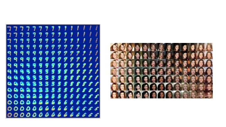
Variational autoencoder (VAE)

latent distribution parameters x = Input(batch_shape=(batch_size, original_dim)) h = Dense(intermediate_dim, activation='relu')(x) z_mean = Dense(latent_dim)(h) z_log_sigma = Dense(latent_dim)(h) def sampling(args): z_mean, z_log_sigma = args epsilon = K. random_normal(shape=(batch_size, latent_dim), mean=0. , std=epsilon_std) return z_mean + K. exp(z_log_sigma) * epsilon # note that "output_shape" isn't necessary with the Tensor. Flow backend # so you could write `Lambda(sampling)([z_mean, z_log_sigma])` z = Lambda(sampling, output_shape=(latent_dim, ))([z_mean, z_log_sigma])

loss def vae_loss(x, x_decoded_mean): xent_loss = objectives. binary_crossentropy(x, x_decoded_mean) kl_loss = - 0. 5 * K. mean(1 + z_log_sigma - K. square(z_mean) - K. exp(z_log_sigma), axis=-1) return xent_loss + kl_loss vae. compile(optimizer='rmsprop', loss=vae_loss)

CVPR 2018 Learned Image Compression Challenge Tasks Dataset P (“professional”) and Dataset M (“mobile”) We will provide two rankings of participants (and baseline image compression methods – Web. P, JPEG 2000, and BPG) based on the following criteria: ● ● PSNR Scores provided by human raters

Resource François Chollet/Deep Learning with Python (ch. 8. 4)

Next ● CNN ● GAN NIPS 2016 Tutorial: Generative Adversarial Networks