Deep Learning 2 Basic Theory of Convolutional Neural

Deep Learning 2: Basic Theory of Convolutional Neural Network Ph. D Student: Li-Wen Wang Supervisor: Professor Wan-Chi Siu and Dr. Daniel Pak-Kong Lun 15 July, 2020 1

v Outline • Introduction • Review: Neural Network (NN) • Convolutional Neural Network (CNN) • Comparison between NN and CNN • Milestones (brief) • • Le. Net (1998) Alex. Net (2012) VGG Net (2014) U-Net (2015) • Deep Convolutional Neural Network • Advantages and Problems of Deep Structure • Res. Net (2015) • Conclusion 2

Part 1: Introduction Ø Review: Neural Network (NN) Ø Convolutional Neural Network (CNN) 3

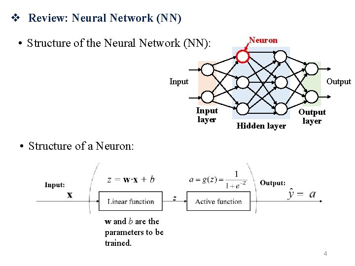
v Review: Neural Network (NN) • Structure of the Neural Network (NN): Neuron Input Output Input layer Hidden layer Output layer • Structure of a Neuron: w and b are the parameters to be trained. 4

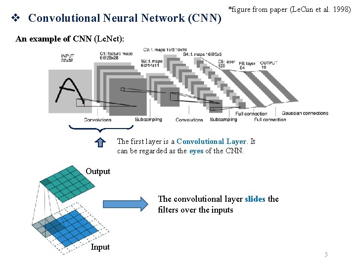
v Convolutional Neural Network (CNN) *figure from paper (Le. Cun et al. 1998) An example of CNN (Le. Net): The first layer is a Convolutional Layer. It can be regarded as the eyes of the CNN. Output The convolutional layer slides the filters over the inputs Input 5

v Convolutional Neural Network (CNN) Convolutional layer: Input x Filter (weight) w Output z b + bias For each time: z = w·x + b · denotes element-wise multiplication +0 6

v Convolutional Neural Network (CNN) Convolutional layer: Input x Filter (weight) w Output z b + bias For the layer: z= w*x + b * denotes convolution 7

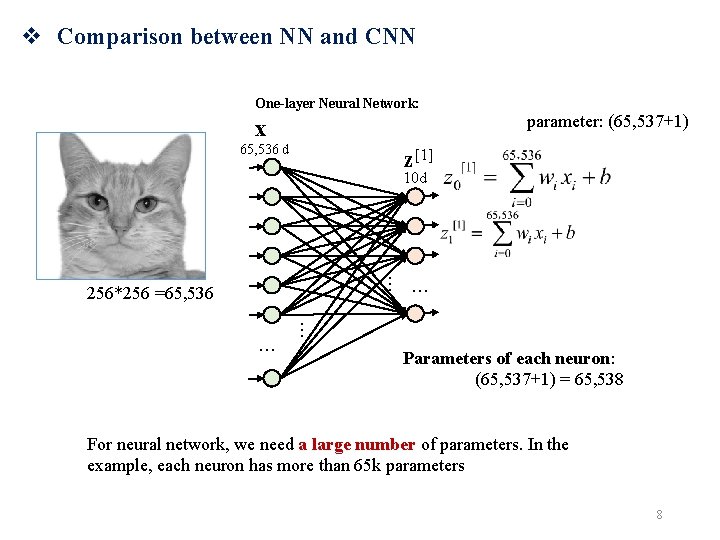
v Comparison between NN and CNN One-layer Neural Network: x 65, 536 d parameter: (65, 537+1) z[1] 10 d … 256*256 =65, 536 … … … Parameters of each neuron: (65, 537+1) = 65, 538 For neural network, we need a large number of parameters. In the example, each neuron has more than 65 k parameters 8

v Comparison between NN and CNN Convolutional layer: Input x Filter (weight) w b + Output z Parameters to be trained: (3*3+1) = 10 bias For image processing task, we can use convolutional neural network to reduce the parameters. If using a 3*3 filter, it needs only 10 parameters to learn. 9

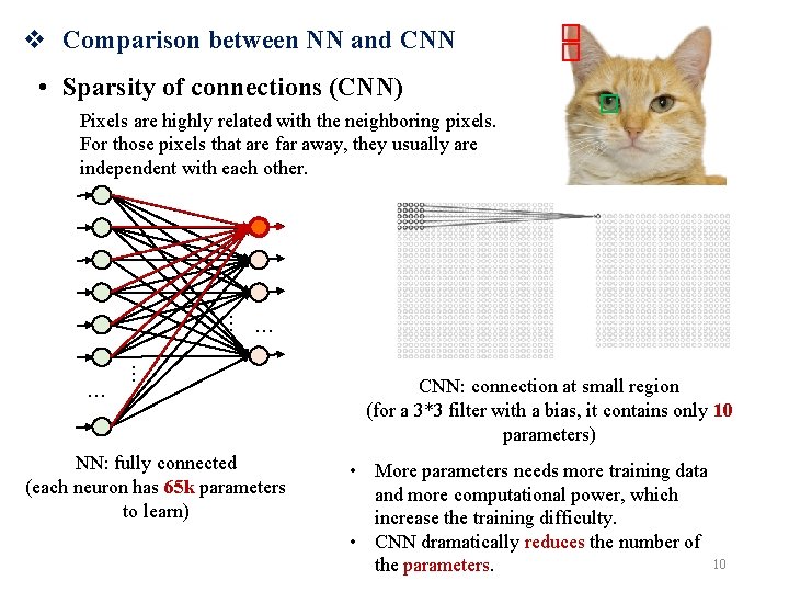
v Comparison between NN and CNN • Sparsity of connections (CNN) Pixels are highly related with the neighboring pixels. For those pixels that are far away, they usually are independent with each other. … … NN: fully connected (each neuron has 65 k parameters to learn) CNN: connection at small region (for a 3*3 filter with a bias, it contains only 10 parameters) • More parameters needs more training data and more computational power, which increase the training difficulty. • CNN dramatically reduces the number of 10 the parameters.

v Convolutional Neural Network • Parameter sharing (CNN) “If detecting a horizontal edge is important at some location in the image, it should intuitively be useful at some other location” -- (cs 231 n, Convolutional Neural Networks for Visual Recognition) Therefore, for the convolutional layer, the parameters are very efficient that makes the training easier. 11

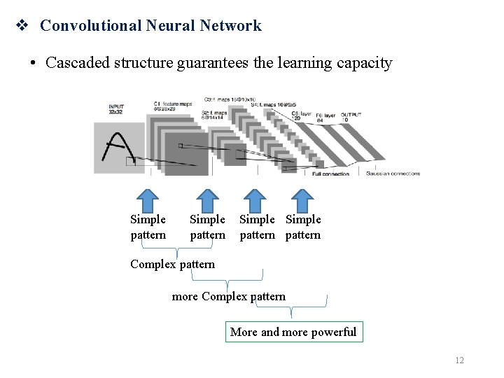
v Convolutional Neural Network • Cascaded structure guarantees the learning capacity Simple pattern Simple pattern Complex pattern more Complex pattern More and more powerful 12

Part 2: Milestones Ø Le. Net (1998) Ø Alex. Net (2012) Ø VGG Net (2014) Ø U-Net (2015) 13

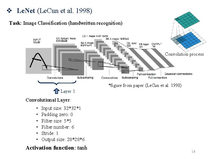
v Le. Net (Le. Cun et al. 1998) Task: Image Classification (handwritten recognition) Convolution process *figure from paper (Le. Cun et al. 1998) Layer 1 Convolutional Layer: • • • Input size: 32*32*1 Padding zero: 0 Filter size: 5*5 Filter number: 6 Stride: 1 Output size: 28*28*6 Activation function: tanh 14

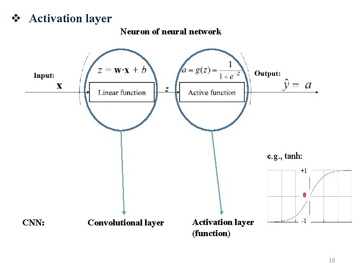
v Activation layer Neuron of neural network e. g. , tanh: +1 0 CNN: Convolutional layer Activation layer (function) -1 16

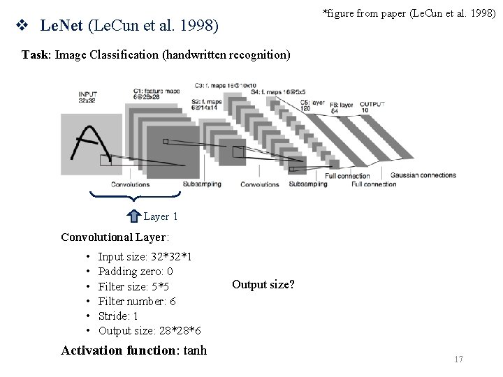
*figure from paper (Le. Cun et al. 1998) v Le. Net (Le. Cun et al. 1998) Task: Image Classification (handwritten recognition) Layer 1 Convolutional Layer: • • • Input size: 32*32*1 Padding zero: 0 Filter size: 5*5 Filter number: 6 Stride: 1 Output size: 28*28*6 Activation function: tanh Output size? 17

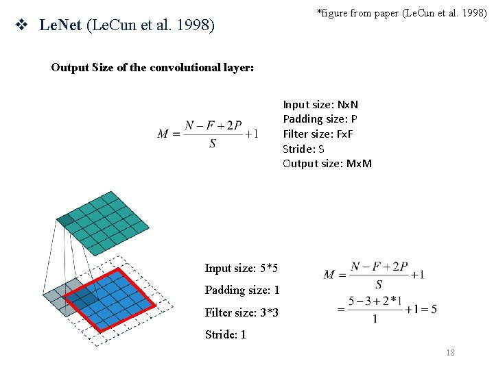
v Le. Net (Le. Cun et al. 1998) *figure from paper (Le. Cun et al. 1998) Output Size of the convolutional layer: Input size: Nx. N Padding size: P Filter size: Fx. F Stride: S Output size: Mx. M Input size: 5*5 Padding size: 1 Filter size: 3*3 Stride: 1 18

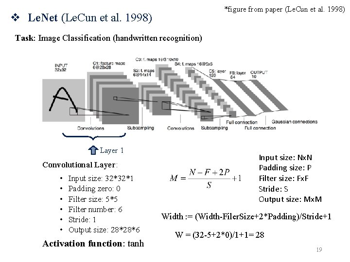
*figure from paper (Le. Cun et al. 1998) v Le. Net (Le. Cun et al. 1998) Task: Image Classification (handwritten recognition) Layer 1 Convolutional Layer: • • • Input size: 32*32*1 Padding zero: 0 Filter size: 5*5 Filter number: 6 Stride: 1 Output size: 28*28*6 Activation function: tanh Input size: Nx. N Padding size: P Filter size: Fx. F Stride: S Output size: Mx. M Width : = (Width-Filer. Size+2*Padding)/Stride+1 W = (32 -5+2*0)/1+1= 28 19

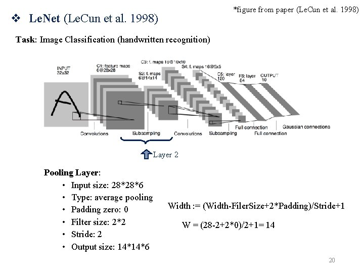
*figure from paper (Le. Cun et al. 1998) v Le. Net (Le. Cun et al. 1998) Task: Image Classification (handwritten recognition) Layer 2 Pooling Layer: • Input size: 28*28*6 • Type: average pooling • Padding zero: 0 • Filter size: 2*2 • Stride: 2 • Output size: 14*14*6 Width : = (Width-Filer. Size+2*Padding)/Stride+1 W = (28 -2+2*0)/2+1= 14 20

v Pooling Layer • Mostly used immediately after the convolutional layer to reduce the spatial size (feature selection). Average pooling: 7 2 6 2 4 5 4 7 Average pooling with 3 3 4 2 2 x 2 filter and stride 2 6 4 8 6 4. 5 4. 75 4 5 7 7 6 8 Maximum pooling: 7 2 6 2 4 5 4 7 Max pooling with 3 3 4 2 2 x 2 filter and stride 2 6 4 8 6 21

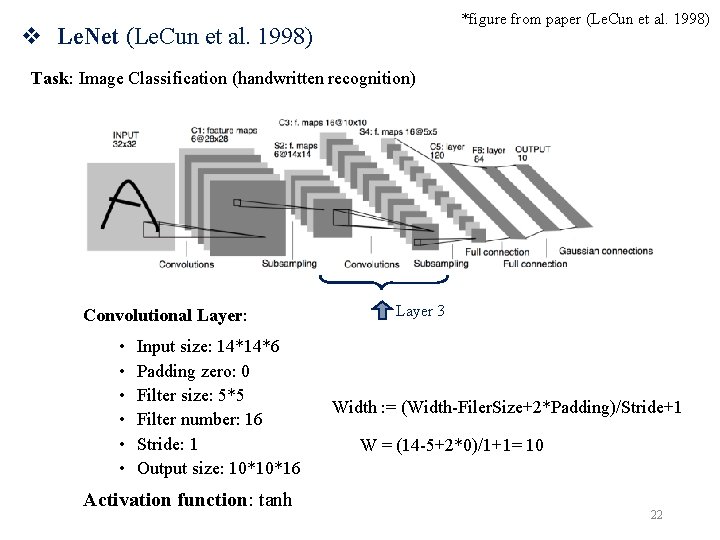
*figure from paper (Le. Cun et al. 1998) v Le. Net (Le. Cun et al. 1998) Task: Image Classification (handwritten recognition) Convolutional Layer: • • • Input size: 14*14*6 Padding zero: 0 Filter size: 5*5 Filter number: 16 Stride: 1 Output size: 10*10*16 Activation function: tanh Layer 3 Width : = (Width-Filer. Size+2*Padding)/Stride+1 W = (14 -5+2*0)/1+1= 10 22

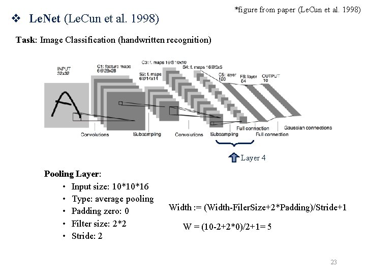
*figure from paper (Le. Cun et al. 1998) v Le. Net (Le. Cun et al. 1998) Task: Image Classification (handwritten recognition) Layer 4 Pooling Layer: • Input size: 10*10*16 • Type: average pooling • Padding zero: 0 • Filter size: 2*2 • Stride: 2 • Output size: 5*5*16 Width : = (Width-Filer. Size+2*Padding)/Stride+1 W = (10 -2+2*0)/2+1= 5 23

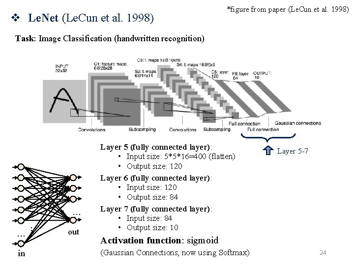
v Le. Net (Le. Cun et al. 1998) *figure from paper (Le. Cun et al. 1998) Task: Image Classification (handwritten recognition) … in … … … out Layer 5 (fully connected layer): • Input size: 5*5*16=400 (flatten) • Output size: 120 Layer 6 (fully connected layer): • Input size: 120 • Output size: 84 Layer 7 (fully connected layer): • Input size: 84 • Output size: 10 Layer 5 -7 Activation function: sigmoid (Gaussian Connections, now using Softmax) 24

v Le. Net (Le. Cun et al. 1998) *figure from paper (Le. Cun et al. 1998) Basic structure: • Conv – Pool – fc – out (It has similar elements as current network) Difference from current network: • Activation function: tanh & sigmoid (gradient vanishing problem) Result on MNIST handwritten digit recognition (error rate) : • 0. 8% (Le. Net), 7. 6%(Linear Classifiers), 5% (KNN), 3. 3%(Non-Linear Classifiers) etc. 25

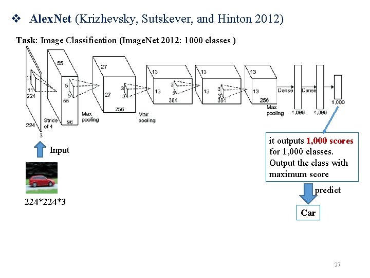
v Alex. Net (Krizhevsky, Sutskever, and Hinton 2012) Task: Image Classification (Image. Net 2012: 1000 classes ) Input it outputs 1, 000 scores for 1, 000 classes. Output the class with maximum score predict 224*3 Car 27

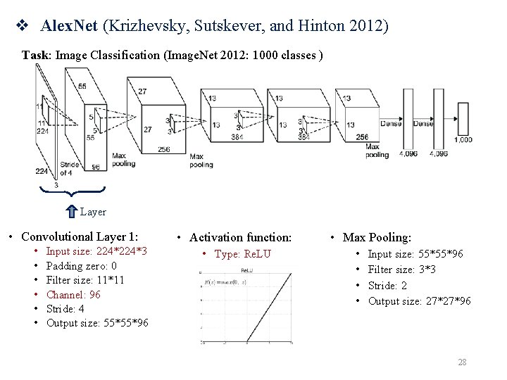
v Alex. Net (Krizhevsky, Sutskever, and Hinton 2012) Task: Image Classification (Image. Net 2012: 1000 classes ) Layer • Convolutional Layer 1: • • • Input size: 224*3 Padding zero: 0 Filter size: 11*11 Channel: 96 Stride: 4 Output size: 55*55*96 • Activation function: • Type: Re. LU • Max Pooling: • • Input size: 55*55*96 Filter size: 3*3 Stride: 2 Output size: 27*27*96 28

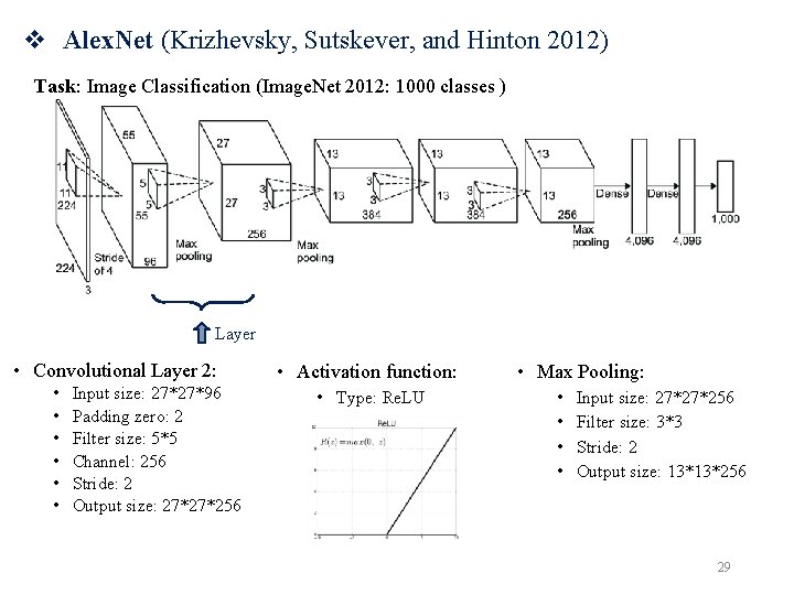
v Alex. Net (Krizhevsky, Sutskever, and Hinton 2012) Task: Image Classification (Image. Net 2012: 1000 classes ) Layer • Convolutional Layer 2: • • • Input size: 27*27*96 Padding zero: 2 Filter size: 5*5 Channel: 256 Stride: 2 Output size: 27*27*256 • Activation function: • Type: Re. LU • Max Pooling: • • Input size: 27*27*256 Filter size: 3*3 Stride: 2 Output size: 13*13*256 29

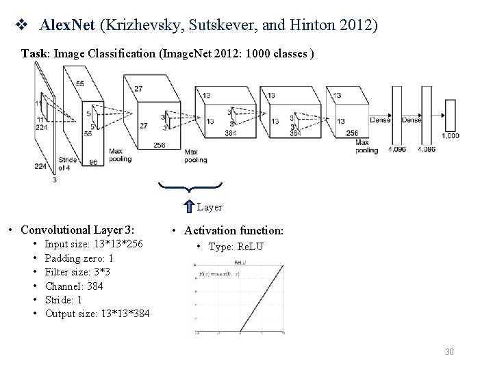
v Alex. Net (Krizhevsky, Sutskever, and Hinton 2012) Task: Image Classification (Image. Net 2012: 1000 classes ) Layer • Convolutional Layer 3: • • • Input size: 13*13*256 Padding zero: 1 Filter size: 3*3 Channel: 384 Stride: 1 Output size: 13*13*384 • Activation function: • Type: Re. LU 30

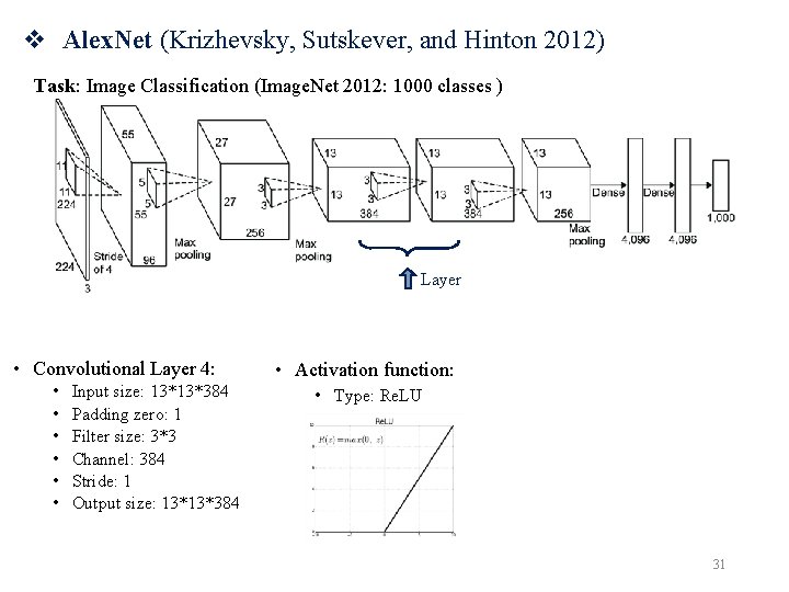
v Alex. Net (Krizhevsky, Sutskever, and Hinton 2012) Task: Image Classification (Image. Net 2012: 1000 classes ) Layer • Convolutional Layer 4: • • • Input size: 13*13*384 Padding zero: 1 Filter size: 3*3 Channel: 384 Stride: 1 Output size: 13*13*384 • Activation function: • Type: Re. LU 31

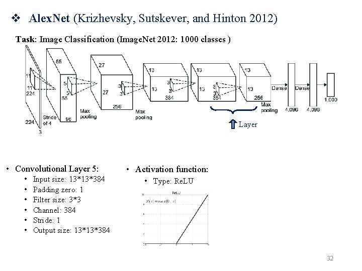
v Alex. Net (Krizhevsky, Sutskever, and Hinton 2012) Task: Image Classification (Image. Net 2012: 1000 classes ) Layer • Convolutional Layer 5: • • • Input size: 13*13*384 Padding zero: 1 Filter size: 3*3 Channel: 384 Stride: 1 Output size: 13*13*384 • Activation function: • Type: Re. LU 32

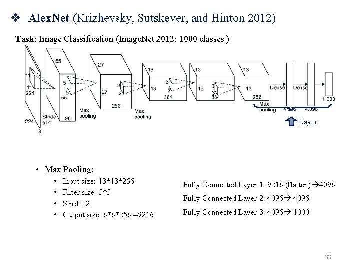
v Alex. Net (Krizhevsky, Sutskever, and Hinton 2012) Task: Image Classification (Image. Net 2012: 1000 classes ) Layer • Max Pooling: • • Input size: 13*13*256 Filter size: 3*3 Stride: 2 Output size: 6*6*256 =9216 Fully Connected Layer 1: 9216 (flatten) 4096 Fully Connected Layer 2: 4096 Fully Connected Layer 3: 4096 1000 33

v Alex. Net (Krizhevsky, Sutskever, and Hinton 2012) Task: Image Classification (Image. Net 2012: 1000 classes ) Result on ILSVRC-2012 image classification competition : • Top-5 error rate of 15. 3%, (second-best entry: 26. 2%) 34

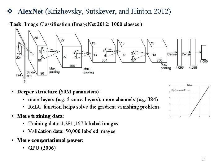
v Alex. Net (Krizhevsky, Sutskever, and Hinton 2012) Task: Image Classification (Image. Net 2012: 1000 classes ) • Deeper structure (60 M parameters) : • more layers (e. g. 5 conv. layers), more channels (e. g. 384) • Re. LU function helps solve the gradient vanishing problem • More training data: • Training data: 1, 281, 167 labeled images • Validation data: 50, 000 labeled images • More computational power: • GPU (2006) 35

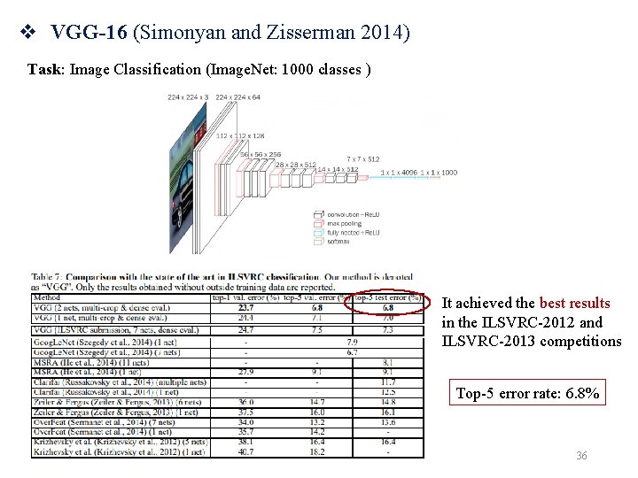
v VGG-16 (Simonyan and Zisserman 2014) Task: Image Classification (Image. Net: 1000 classes ) It achieved the best results in the ILSVRC-2012 and ILSVRC-2013 competitions Top-5 error rate: 6. 8% 36

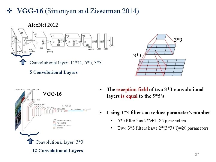
v VGG-16 (Simonyan and Zisserman 2014) Alex. Net 2012 3*3 Convolutional layer: 11*11, 5*5, 3*3 5 Convolutional Layers VGG-16 • The reception field of two 3*3 convolutional layers is equal to the 5*5’s. • Using 3*3 filter can reduce parameter’s number. • 5*5 filter has 5*5+1=26 parameters • Two 3*3 filters have 2*(3*3+1)=20 parameters Convolutional layer: 3*3 12 Convolutional Layers 37

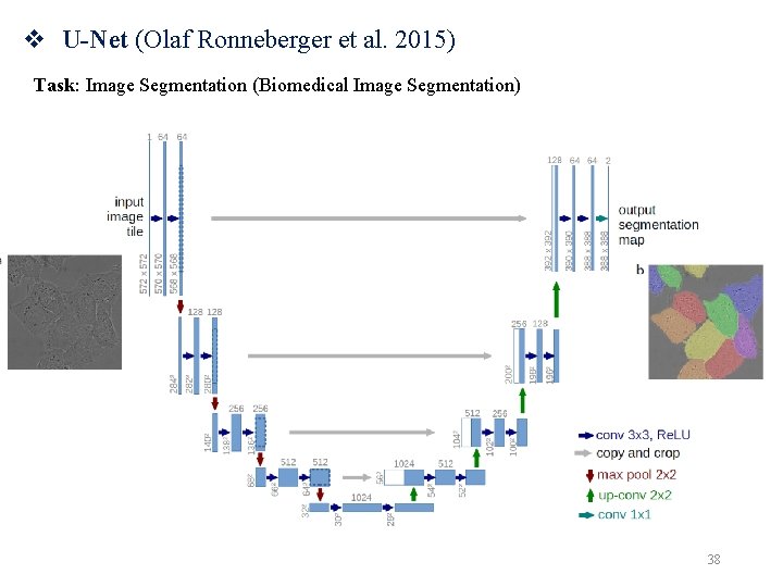
v U-Net (Olaf Ronneberger et al. 2015) Task: Image Segmentation (Biomedical Image Segmentation) 38

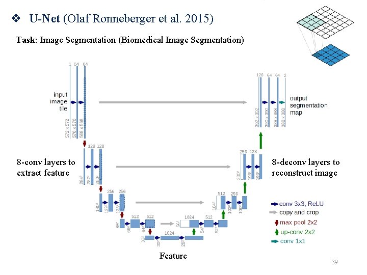
v U-Net (Olaf Ronneberger et al. 2015) Task: Image Segmentation (Biomedical Image Segmentation) 8 -conv layers to extract feature 8 -deconv layers to reconstruct image Feature 39

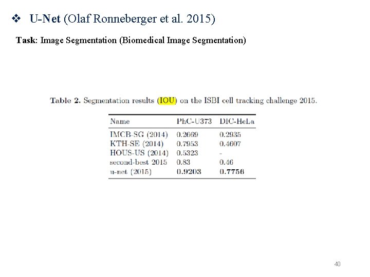
v U-Net (Olaf Ronneberger et al. 2015) Task: Image Segmentation (Biomedical Image Segmentation) 40

Part 3: Deep Convolutional Neural Network Ø Advantages and problem of deep structure Ø Res. Net (2016) 41

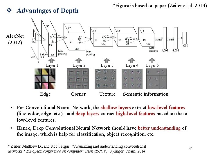
v Advantages of Depth *Figure is based on paper (Zeiler et al. 2014) Alex. Net (2012) Layer 1 Edge Layer 2 Layer 3 Corner Texture Layer 4 Layer 5 Semantic information • For Convolutional Neural Network, the shallow layers extract low-level features (like color, edge, etc. ) , and deep layers extract high-level features based on these low-level features. • Hence, Deep Convolutional Neural Network should have better understanding of the image, which is help for classification, object recognition, etc. * Zeiler, Matthew D. , and Rob Fergus. "Visualizing and understanding convolutional networks. " European conference on computer vision (ECCV). Springer, Cham, 2014. 42

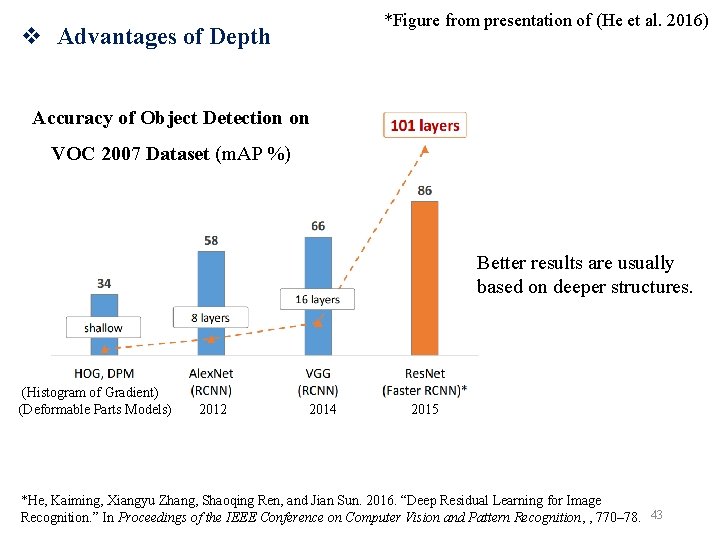
*Figure from presentation of (He et al. 2016) v Advantages of Depth Accuracy of Object Detection on VOC 2007 Dataset (m. AP %) Better results are usually based on deeper structures. (Histogram of Gradient) (Deformable Parts Models) 2012 2014 2015 *He, Kaiming, Xiangyu Zhang, Shaoqing Ren, and Jian Sun. 2016. “Deep Residual Learning for Image Recognition. ” In Proceedings of the IEEE Conference on Computer Vision and Pattern Recognition, , 770– 78. 43

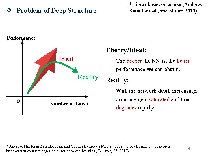
* Figure based on course (Andrew, Katanforoosh, and Mourri 2019) v Problem of Deep Structure Performance Theory/Ideal: Ideal The deeper the NN is, the better performance we can obtain. Reality Number of Layer Reality: With the network depth increasing, accuracy gets saturated and then degrades rapidly. * Andrew, Ng, Kian Katanforoosh, and Younes Bensouda Mourri. 2019. “Deep Learning. ” Coursera. https: //www. coursera. org/specializations/deep-learning (February 23, 2019). 44

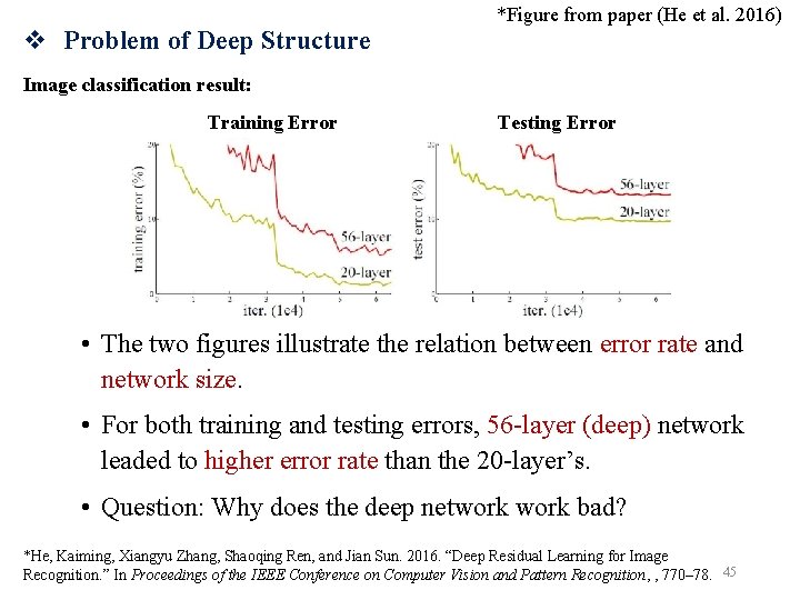
v Problem of Deep Structure *Figure from paper (He et al. 2016) Image classification result: Training Error Testing Error • The two figures illustrate the relation between error rate and network size. • For both training and testing errors, 56 -layer (deep) network leaded to higher error rate than the 20 -layer’s. • Question: Why does the deep network bad? *He, Kaiming, Xiangyu Zhang, Shaoqing Ren, and Jian Sun. 2016. “Deep Residual Learning for Image Recognition. ” In Proceedings of the IEEE Conference on Computer Vision and Pattern Recognition, , 770– 78. 45

v Problem of Deep Structure (reason) • Gradient descent a[0] Slope ranges from 0 to 0. 25 a[1] a[2] a[3] a[4] 0. 5 0. 000005 • Chain Rule Gradient vanishing 0. 1 0. 00001 e. g. 0. 1 46

v Problem of Deep Structure (reason) • Gradient descent a[0] a[1] a[2] a[3] a[4] 0. 5 5000 • Chain Rule Gradient exploding 10 10 e. g. 10 10000 1 47

v Problem of Deep Structure (reason) *Figure from paper of (He et al. 2016) 34 -layer plain network: Gradient Loss Each rectangular is a convolutional layer Difficult to train • Chain Rule Gradient vanishing/exploding problem 48

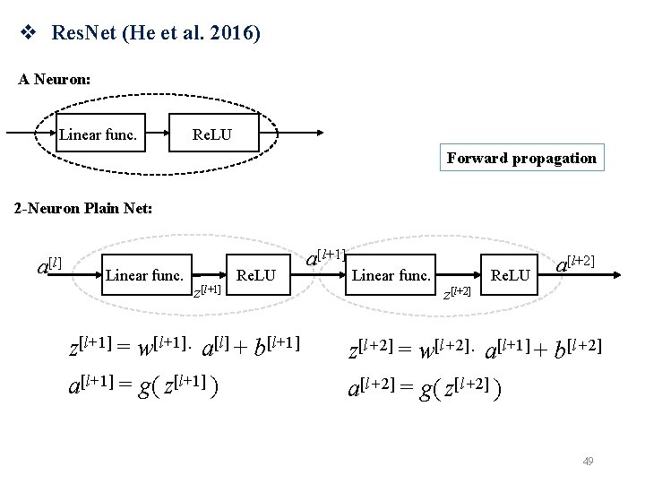
v Res. Net (He et al. 2016) A Neuron: Linear func. Re. LU Forward propagation 2 -Neuron Plain Net: a[l] Linear func. z[l+1] Re. LU a[l+1] Linear func. Re. LU a[l+2] z[l+1] = w[l+1]· a[l] + b[l+1] z[l+2] = w[l+2]· a[l+1] + b[l+2] a[l+1] = g( z[l+1] ) a[l+2] = g( z[l+2] ) 49

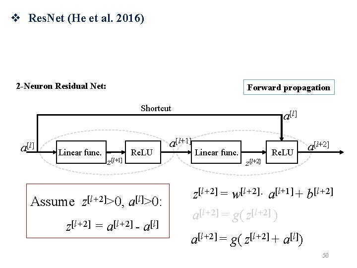
v Res. Net (He et al. 2016) 2 -Neuron Residual Net: Forward propagation Shortcut a[l] Linear func. z[l+1] Re. LU a[l] a[l+1] [l] + b[l+1] z[l+1] = w[l+1] · a Assume z[l+2]>0, a[l]>0: a[l+1] = g( z[l+1] ) z[l+2] = a[l+2] - a[l] Linear func. Re. LU a[l+2] z[l+2] = w[l+2]· a[l+1] + b[l+2] a[l+2] = g( z[l+2] ) a[l+2] = g( z[l+2] + a[l]) 50

v Res. Net (He et al. 2016) Re. LU Backward propagation Gradient Shortcut a[l] Linear func. z[l+1] Re. LU a[l+1] Gradient a[l] Linear func. Re. LU a[l+2] Loss z[l+2] a[l+2] = g( z[l+2] + a[l]) Gradient vanishing 1 Solved ! 51

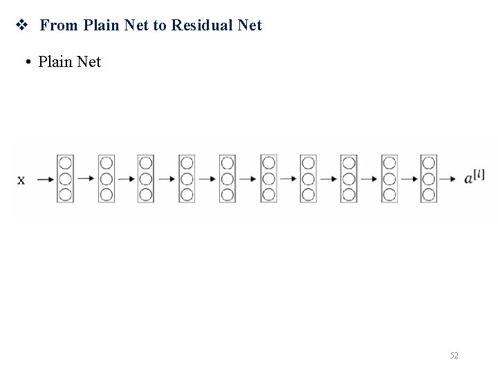
v From Plain Net to Residual Net • Plain Net 52

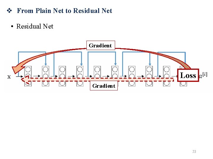
v From Plain Net to Residual Net • Residual Net Gradient Loss Gradient 53

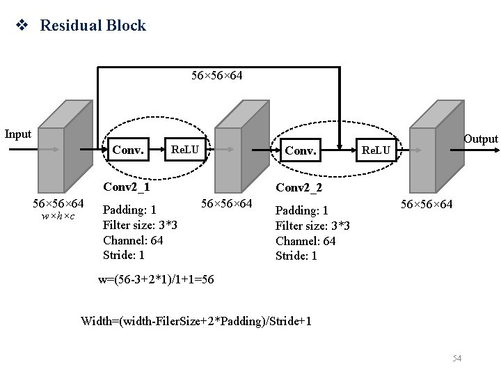
v Residual Block 56× 64 Input Conv. Re. LU Conv 2_1 56× 64 w×h×c Padding: 1 Filter size: 3*3 Channel: 64 Stride: 1 Output Re. LU Conv 2_2 56× 64 Padding: 1 Filter size: 3*3 Channel: 64 Stride: 1 56× 64 w=(56 -3+2*1)/1+1=56 Width=(width-Filer. Size+2*Padding)/Stride+1 54

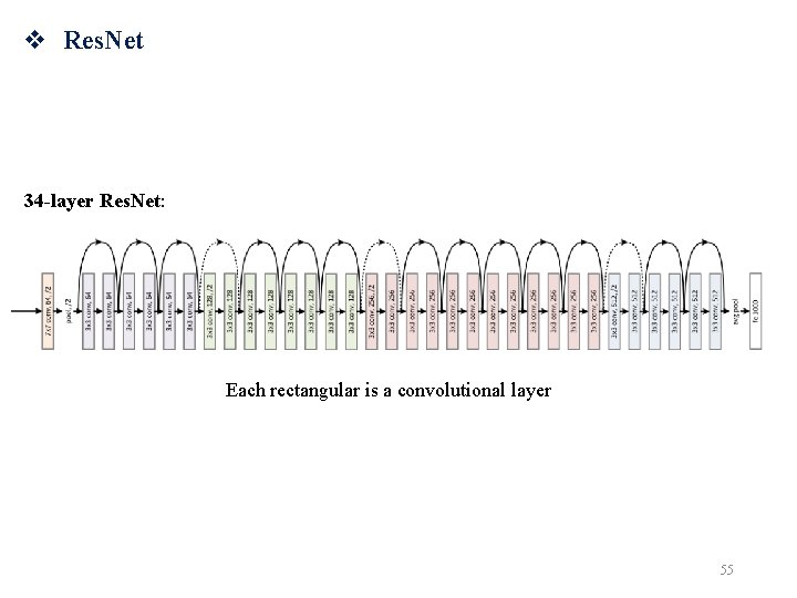
v Res. Net 34 -layer plain Res. Net: network: Each rectangular is a convolutional layer 55

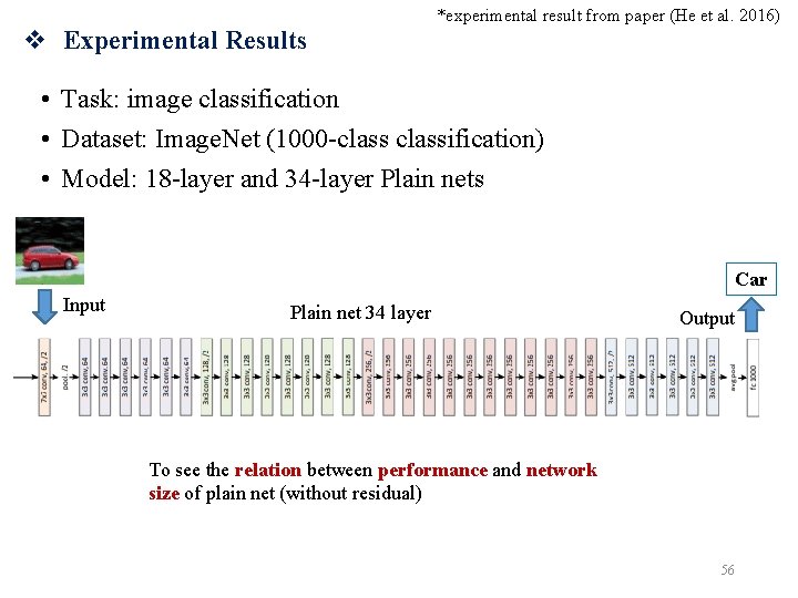
v Experimental Results *experimental result from paper (He et al. 2016) • Task: image classification • Dataset: Image. Net (1000 -classification) • Model: 18 -layer and 34 -layer Plain nets Car Input Plain net 34 layer Plain net 18 layer Output To see the relation between performance and network size of plain net (without residual) 56

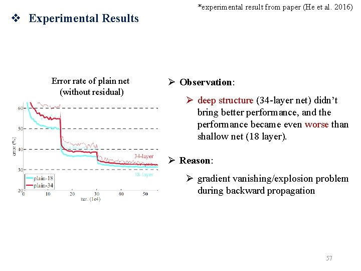
v Experimental Results Error rate of plain net (without residual) *experimental result from paper (He et al. 2016) Ø Observation: Ø deep structure (34 -layer net) didn’t bring better performance, and the performance became even worse than shallow net (18 layer). Ø Reason: Ø gradient vanishing/explosion problem during backward propagation 57

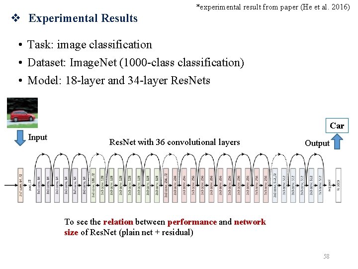
v Experimental Results *experimental result from paper (He et al. 2016) • Task: image classification • Dataset: Image. Net (1000 -classification) • Model: 18 -layer and 34 -layer Res. Nets Car Input Res. Net with 18 convolutional layers Res. Net with 36 convolutional layers Output To see the relation between performance and network size of Res. Net (plain net + residual) 58

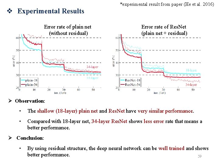
v Experimental Results Error rate of plain net (without residual) *experimental result from paper (He et al. 2016) Error rate of Res. Net (plain net + residual) Ø Observation: • The shallow (18 -layer) plain net and Res. Net have very similar performance. • Compared with 18 -layer net, 34 -layer Res. Net shows less error rate that means a better performance. Ø Conclusion: • By using residual structure, the deep neural network can be well trained and shows better performance. 59

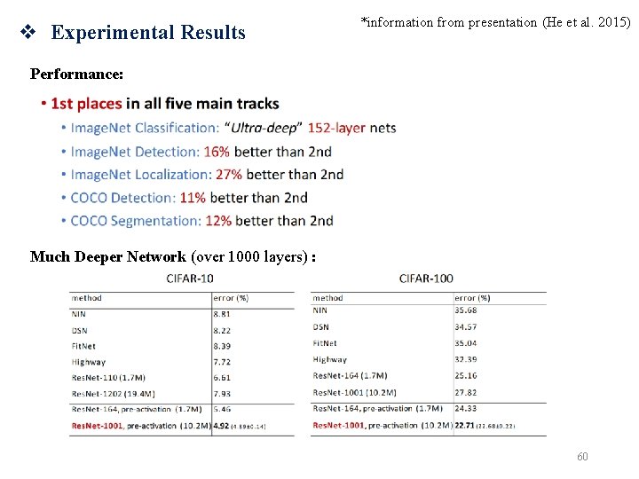
v Experimental Results *information from presentation (He et al. 2015) Performance: Much Deeper Network (over 1000 layers) : 60

v Conclusion • We present the DNN and CNN structure • We briefly shows some famous CNN works (structure, improvements, performance) • Difficulty of training DNN and shows a good solution (Res. Net) 61

v Reference • He, Kaiming, Xiangyu Zhang, Shaoqing Ren, and Jian Sun. 2016. “Deep Residual Learning for Image Recognition. ” In Proceedings of the IEEE Conference on Computer Vision and Pattern Recognition, , 770– 78. • Hinton, Geoffrey E, and Ruslan R Salakhutdinov. 2006. “Reducing the Dimensionality of Data with Neural Networks. ” science 313(5786): 504– 7. • Krizhevsky, Alex, Ilya Sutskever, and Geoffrey E Hinton. 2012. “Imagenet Classification with Deep Convolutional Neural Networks. ” In Advances in Neural Information Processing Systems, , 1097– 1105. • Le. Cun, Yann, Léon Bottou, Yoshua Bengio, and Patrick Haffner. 1998. “Gradient. Based Learning Applied to Document Recognition. ” Proceedings of the IEEE 86(11): 2278– 2324. • Simonyan, Karen, and Andrew Zisserman. 2014. “Very Deep Convolutional Networks for Large-Scale Image Recognition. ” ar. Xiv preprint ar. Xiv: 1409. 1556. • Andrew, Ng, Kian Katanforoosh, and Younes Bensouda Mourri. 2019. “Deep Learning. ” Coursera. https: //www. coursera. org/specializations/deep-learning (February 23, 2019). 62

• The end, thank you! 63