Deep Inelastic Scattering DIS Parton Distribution Functions and
: Parton Distribution Functions and low-x physics Goa Sept 2008 A.")
Deep Inelastic Scattering (DIS): Parton Distribution Functions and low-x physics Goa Sept 2008 A. M. Cooper-Sarkar Oxford What have we learnt from DIS in the last 30 years? QPM, QCD Parton Distribution Functions, αs Low-x physics

PDFs were first investigated in deep inelastic lepton-hadron scatterning -DIS Lμν Wμν dσ ~ E’ q = k – k’, Q 2 = -q 2 Ee Ep Px = p + q , W 2 = (p + q)2 s= (p + k)2 x = Q 2 / (2 p. q) y = (p. q)/(p. k) W 2 = Q 2 (1/x – 1) Q 2 = s x y s = 4 Ee Ep Q 2 = 4 Ee E’ sin 2θe/2 y = (1 – E’/Ee cos 2θe/2) x = Q 2/sy 2 Leptonic tensor calculable The kinematic variables are measurable Hadronic tensorconstrained by Lorentz invariance
 = [")
Completely generally the double differential cross-section for e-N scattering d 2 (e±N) = [ Y+ F 2(x, Q 2) - y 2 FL(x, Q 2) ± Y_x. F 3(x, Q 2)], Y± = 1 ± (1 -y)2 dxdy Leptonic part hadronic part F 2, FL and x. F 3 are structure functions which express the dependence of the cross-section on the structure of the nucleon– The Quark-Parton model interprets these structure functions as related to the momentum distributions of quarks or partons within the nucleon AND the measurable kinematic variable x = Q 2/(2 p. q) is interpreted as the FRACTIONAL momentum of the incoming nucleon taken by the struck quark (x. P+q)2=x 2 p 2+q 2+2 xp. q ~ 0 for massless quarks and p 2~0 so x = Q 2/(2 p. q) The FRACTIONAL momentum of the incoming nucleon taken by the struck quark is the MEASURABLE quantity x
![Consider electron muon scattering d = 2 2 s [ 1 + (1 -y)2]](http://slidetodoc.com/presentation_image_h/ea3ab76ab654dd34cc2278922aba9612/image-4.jpg "Consider electron muon scattering d = 2 2 s [ 1 + (1 -y)2]")
Consider electron muon scattering d = 2 2 s [ 1 + (1 -y)2] , for elastic eμ dy Q 4 isotropic non-isotropic d = 2 2 ei 2 s [ 1 + (1 -y)2] , so for elastic electron quark scattering, quark charge ei e dy d 2 dxdy Q 4 = 2 2 s [ 1 + (1 -y)2] Σi ei 2(xq(x) + xq(x))so for e. N, where eq has c. of m. energy 2 equal to xs, and q(x) gives probability that such a quark is in the Nucleon Q 4 Now compare the general equation to the QPM prediction to obtain the results F 2(x, Q 2) = Σi ei 2(xq(x) + xq(x)) – Bjorken scaling – this depends only on x FL(x, Q 2) = 0 - spin ½ quarks x. F 3(x, Q 2) = 0 - only γ exchange
= GF 2 x s dy")
Consider , scattering: neutrinos are handed d ( )= GF 2 x s dy For q (left-left) d ( ) = GF 2 x s (1 -y)2 Compare to the general form of the crosssection for n/n scattering via W+/- dy FL (x, Q 2) = 0 For q (left-right) x. F 3(x, Q 2) = 2Σix(qi(x) - qi(x)) d 2 ( ) = GF 2 s Σi [xqi(x) +(1 -y)2 xqi(x)] dxdy Valence For N F 2(x, Q 2) = 2Σix(qi(x) + qi(x)) d 2 ( ) = GF 2 s Σi [xqi(x) +(1 -y)2 xqi(x)] dxdy Clearly there antiquarks in the nucleon Valence and Sea For N 3 Valence quarks plus a flavourless qq Sea And there will be a relationship between F 2 e. N and F 2 n. N Also NOTE n, n scattering is FLAVOUR sensitive - W+ u W+ can only hit quarks of charge -e/3 or antiquarks -2 e/3 d ( p) ~ (d + s) + (1 - y)2 (u + c) ( p) ~ (u + c) (1 - y)2 + (d + s) q = qvalence +qsea q = qsea= qsea

So in , scattering the sums over q, qbar ONLY contain the appropriate flavours BUThigh statistics , data are taken on isoscalar targets e. g. Fe ~ (p + n)/2=N d in proton = u in neutron u in proton = d in neutron GLS sum rule Total momentum of quarks A TRIUMPH (and 20 years of understanding the c c contribution)

BUT – Bjorken scaling is broken F 2 does not depend only on x it also depends on Q 2 – ln(Q 2) Particularly strongly at small x

QCD improves the Quark Parton Model What if y x or x y Before the quark is struck? Pqq Pqg Pgq Pgg y > x, z = x/y So F 2(x, Q 2) = Σi ei 2(xq(x, Q 2) + xq(x, Q 2)) in LO QCD The theory predicts the rate at which the parton distributions (both quarks and gluons) evolve with Q 2 - (the energy scale of the probe) -BUT it does not predict their shape The DGLAP parton evolution equations
 ~ αs ln. Q 2, but αs(Q 2)~1/ln. Q 2,")
Note q(x, Q 2) ~ αs ln. Q 2, but αs(Q 2)~1/ln. Q 2, so αs ln. Q 2 is O(1), so we must sum all terms What if higher orders are needed? αsn ln. Q 2 n s s(Q 2) Leading Log Approximation x decreases from target to probe xi-1> xi+1…. pt 2 of quark relative to proton increases from target to probe Pqq(z) = P 0 qq(z) + αs P 1 qq(z) +αs 2 P 2 qq(z) LO NNLO pt 2 i-1 < pt 2 i < pt 2 i+1 Dominant diagrams have STRONG pt ordering F 2 is no longer so simply expressed in terms of partons convolution with coefficient functions is needed – but these are calculable in QCD FL is no longer zero. . And it depends on the gluon
")
How do we determine Parton Distribution Functions ? Parametrise the parton distribution functions (PDFs) at Q 20 (~1 -7 Ge. V 2)- Use NLO QCD DGLAP equations to evolve these PDFs to Q 2 >Q 20 Construct the measurable structure functions and cross-sections by convoluting PDFs with coefficient functions: make predictions for ~2000 data points across the x, Q 2 plane- Perform χ2 fit to the data Formalism NLO DGLAP MSbar factorisation Q 0 2 functional form @ Q 02 sea quark (a)symmetry etc. Data DIS (SLAC, BCDMS, NMC, E 665, CCFR, H 1, ZEUS, CCFR, Nu. Te. V ) Drell-Yan (E 605, E 772, E 866, …) High ET jets (CDF, D 0) W rapidity asymmetry (CDF) etc. fi (x, Q 2) αS(MZ ) Who? Alekhin, CTEQ, MRST, H 1, ZEUS http: //durpdg. dur. ac. uk/hepdata/ http: //projects. hepforge. org/lhapdf/ LHAPDFv 5

The DATA – the main contribution is DIS data Terrific expansion in measured range across the x, Q 2 plane throughout the 90’s HERA data Pre HERA fixed target p, D NMC, BDCMS, E 665 and , bar Fe CCFR We have to impose appropriate kinematic cuts on the data so as to remain in the region when the NLO DGLAP formalism is valid 1. Q 2 cut : Q 2 > few Ge. V 2 so that perturbative QCD is applicable- αs(Q 2) small 2. W 2 cut: to avoid higher twist terms- usual formalism is leading twist 3. x cut: to avoid regions where ln(1/x) resummation (BFKL) and non-linear effects may be necessary….

Need to extend the formalism? Optical theorem 2 The handbag diagram- QPM Im QCD at LL(Q 2) Ordered gluon ladders (αsn ln. Q 2 n) NLL(Q 2) one rung disordered αsn ln. Q 2 n-1 And what about Higher twist diagrams ? Are they always subdominant? Important at high x, low Q 2 BUT what about completely disordered Ladders? ? at small x there may be a need for BFKL ln(1/x) resummation?

The strong rise in the gluon density at small-x leads to speculation that there may be a need for non-linear equations? - gluons recombining gg→g Non-linear fan diagrams form part of possible higher twist contributions at low x- no sign of these in data

The CUTS In practice it has been amazing how low in Q 2 the standard formalism still works- down to Q 2 ~ 1 Ge. V 2 : cut Q 2 > 2 Ge. V 2 is typical It has also been surprising how low in x – down to x~ 10 -5 : no x cut is typical Nevertheless there are doubts as to the applicability of the formalism at such low-x. . (See later) there could be ln(1/x) corrections and/or non-linear high density corrections for x < 5 10 -3

Higher twist terms can be important at low-Q 2 and high-x → this is the fixed target region (particularly SLAC- and now JLAB data). Kinematic target mass corrections and dynamic contributions ~ 1/Q 2 X→ 2 x/(1 + √(1+4 m 2 x 2/Q 2)) Fit with F 2=F 2 LT (1 +D 2(x)/Q 2) Fits establish that higher twist terms are not needed if W 2 > 15 Ge. V 2 – typical W 2 cut
 at Q 20")
The form of the parametrisation Parametrise the parton distribution functions (PDFs) at Q 20 (~1 -7 Ge. V 2) Parameters Ag, Au, Ad are fixed through xuv(x) =Auxau (1 -x)bu (1+ εu √x + γu x) momentum and number sum rules – other parameters may be fixed by model xdv(x) =Adxad (1 -x)bd (1+ εd √x + γd x) x. S(x) =Asx-λs (1 -x)bs (1+ εs √x + γs x) xg(x) =Ag x-λg(1 -x)bg (1+ εg √x + γg x) These parameters control the low-x control the middling-x shape These parameters control the high-x shape Alternative form for CTEQ xf(x) = A 0 x. A 1(1 -x)A 2 e. A 3 x (1+e. A 4 x)A 5 choices- Model choices Form of parametrization at Q 20, value of Q 20, , flavour structure of sea, cuts applied, heavy flavour scheme → typically ~15 -22 parameters Use QCD to evolve these PDFs to Q 2 >Q 20 Construct the measurable structure functions by convoluting PDFs with coefficient functions: make predictions for ~2000 data points across the x, Q 2 plane Perform χ2 fit to the data The fact that so few parameters allows us to fit so many data points established QCD as the THEORY OF THE STRONG INTERACTION and provided the first measurements of s (as one of the fit parameters)

The form of the parametrisation at Q 20 Ultimately we may get this from lattice QCD, or other models- the statistical model is quite successful (Soffer et al). But we can make some guesses at the basic form: xa (1 -x)b …. . at one time (20 years ago? ) we thought we understood it! ----the high x power from counting rules ----(1 -x)2 ns-1 - ns spectators valence (1 -x) 3, sea (1 -x)7, gluon (1 -x)5 ----the low-x power from Regge – low-x corresponds to high centre of mass energy for the virtual boson proton collision (x = Q 2 / (2 p. q)) -----Regge theory gives high energy cross-sections as s (α-1) ------which gives x dependence x (1 -α), where α is the intercept of the Regge trajectorydifferent for singlet (no overall flavour) F 2 ~x 0 and non-singlet (flavour- valence -like) x. F 3~x 0. 5 The shapes of F 2 and x. F 3 even looked as if they followed these shapes – pre HERA

But at what Q 2 would these be true? – Valence distributions evolve slowly but sea and gluon distributions evolve fast. We input non-perturbative ideas about shapes at a low scale, but we are just parametrising our ignorance. It turns out that we need the arbitrary polynomial In any case the further you evolve in Q 2 the less the parton distributions look like the low Q 2 inputs and the more they are determined by QCD evolution –Valence distributions evolve slowly Sea/Gluon distributions evolve fast (Some people don’t use a starting parametrization at all- but let neural nets learn the shape of the data- NNPDF)

Where is the information coming from? Originally- pre HERA Assuming u in proton = d in neutron – strong. F 2(e/ p)~ 4/9 x(u +ubar) +1/9 x(d+dbar) + 4/9 x(c +cbar) +1/9 x(s+sbar) isospin Fixed target e/μ p/D data from NMC, BCDMS, E 665, SLAC F 2(e/ D)~5/18 x(u+ubar+d+dbar) + 4/9 x(c +cbar) +1/9 x(s+sbar) Also use ν, νbar fixed target data from CCFR( now also Nu. Te. V/Chorus) (Beware Fe target needs nuclear corrections) F 2(ν, νbar N) = x(u +ubar + dbar + s +sbar + cbar) x. F 3(ν, νbar N) = x(uv + dv ) (provided s = sbar) Valence information for 0< x < 1 Can get ~4 distributions from this: e. g. u, d, ubar, dbar – but need assumptions like q=qbar for all flavours, sbar = 1/4 (ubar+dbar) and heavy quark treatment. Note gluon enters only indirectly via DGLAP equations for evolution
 symmetric sea was assumed u=uv+usea, d=dv+dsea usea= ubar =")
Flavour structure Historically an SU(3) symmetric sea was assumed u=uv+usea, d=dv+dsea usea= ubar = dsea = dbar = sbar =K and c=cbar=0 Measurements of F 2μn = uv + 4 dv +4/3 K F 2μp 4 uv+ dv +4/3 K Establish no valence quarks at small-x F 2μn/F 2μp → 1 But F 2μn/F 2μp → 1/4 as x → 1 Not to 2/3 as it would for dv/uv=1/2, hence it look s as if dv/uv → 0 as x → 1 i. e the dv momentum distribution is softer than that of uv. Why? Non-perturbative physics --diquark structures? How accurate is this? Could dv/uv → 1/4 (Farrar and Jackson)?

Flavour structure in the sea dbar ≠ubar in the sea Consider the Gottfried sum-rule (at LO) ∫ dx (F 2 p-F 2 n) = 1/3 ∫dx (uv-dv) +2/3∫dx(ubar-dbar) If ubar=dbar then the sum should be 0. 33 the measured value from NMC = 0. 235 ± 0. 026 Clearly dbar > ubar…why? low Q 2 non-perturbative effects, sbar≠(ubar+dbar)/2, Pauli blocking, p →nπ+, pπ0, Δ++π - W+ in fact sbar ~ (ubar+dbar)/4 Why? The mass of the strange quark is larger than that of the light quarks Evidence – neutrino opposite sign dimuon production rates And even s≠sbar? Because of p→ΛK+ s c→s μ+ν

So what did HERA bring? Low-x – within conventional NLO DGLAP Before the HERA measurements most of the predictions for low-x behaviour of the structure functions and the gluon PDF were wrong HERA ep neutral current (γ-exchange) data give much more information on the sea and gluon at small x…. . x. Sea directly from F 2, F 2 ~ xq x. Gluon from scaling violations d. F 2 /dln. Q 2 – the relationship to the gluon is much more direct at small-x, d. F 2/dln. Q 2 ~ Pqg xg

Low-x t = ln Q 2/ 2 Gluon splitting functions become singular At small x, small z=x/y xg(x, Q 2) ~ x -λg αs ~ 1/ln Q 2/ 2 A flat gluon at low Q 2 becomes very steep AFTER Q 2 evolution AND F 2 becomes gluon dominated F 2(x, Q 2) ~ x -λs, And yet people didn’t expect this…. See later λs=λg - ε

High Q 2 HERA data-still to be fully exploited HERA data have also provided information at high Q 2 → Z 0 and W+/- become as important as γ exchange → NC and CC cross-sections comparable For NC processes F 2 = i Ai(Q 2) [xqi(x, Q 2) + xqi(x, Q 2)] x. F 3= i Bi(Q 2) [xqi(x, Q 2) - xqi(x, Q 2)] Ai(Q 2) = ei 2 – 2 ei vi ve PZ + (ve 2+ae 2)(vi 2+ai 2) PZ 2 Bi(Q 2) = – 2 e i a e PZ + 4 ai ae vi ve PZ 2 = Q 2/(Q 2 + M 2 Z) 1/sin 2θW a new valence structure function x. F 3 due to Z exchange is measurable from low to high x- on a pure proton target → no heavy target corrections- no assumptions about strong isospin
 = GF 2 M 4 W")
CC processes give flavour information d 2 (e-p) = GF 2 M 4 W [x (u+c) + (1 -y)2 x (d+s)] dxdy 2 x(Q 2+M 2 W)2 MW information uv at high x d 2 (e+p) = GF 2 M 4 W [x (u+c) + (1 -y)2 x (d+s)] dxdy 2 x(Q 2+M 2 W)2 dv at high x Measurement of high-x dv on a pure proton target d is not well known because u couples more strongly to the photon. Historically information has come from deuterium targets –but even Deuterium needs binding corrections. Open questions: does u in proton = d in neutron? , does dv/uv 0, as x 1?

How has our knowledge evolved?

To reveal the difference in both large and small x regions The u quark LO fits to early fixed-target DIS data To view small and large x in one plot

Rise from HERA data

The story about the gluon is more complex Gluon

Gluon HERA steep rise of F 2 at low x

Gluon More recent fits with HERA data - steep rise even for low Q 2 ~ 1 Ge. V 2 Tev jet data Does gluon go negative at small x and low Q? see MRST/W PDFs

PDF comparison 2008 The latest HERAPDF 0. 1 gives very small experimental errors and modest model errors

Modern analyses assess PDF uncertainties within the fit Clearly errors assigned to the data points translate into errors assigned to the fit parameters -and these can be propagated to any quantity which depends on these parameters— the parton distributions or the structure functions and crosssections which are calculated from them < б 2 F > = Σj Σk ∂ F Vjk ∂ F ∂ pj ∂ pk The errors assigned to the data are both statistical and systematic and for much of the kinematic plane the size of the pointto-point correlated systematic errors is ~3 times the statistical errors This must be treated carefully in the χ2 definition

Some data sets incompatible/only marginally compatible? One could restrict the data sets to those which are sufficiently consistent that these problems do not arise – (H 1, GKK, Alekhin) But one loses information since partons need constraints from many different data sets – noone experiment has sufficient kinematic range / flavour information (though HERA comes close) To illustrate: the χ2 for the MRST global fit is plotted versus the variation of a particular parameter (αs ). The individual χ2 e for each experiment is also plotted versus this parameter in the neighbourhood of the global minimum. Each experiment favours a different value of. αs PDF fitting is a compromise. Can one evaluate acceptable ranges of the parameter value with respect to the individual experiments?

Distance illustration for eigenvector-4 CTEQ 6 look at eigenvector combinations of their parameters rather than the parameters themselves. They determine the 90% C. L. bounds on the distance from the global minimum from ∫ P(χe 2, Ne) dχe 2 =0. 9 for each experiment This leads them to suggest a modification of the χ2 tolerance, Δχ2 = 1, with which errors are evaluated such that Δχ2 = T 2, T = 10. Why? Pragmatism. The size of the tolerance T is set by considering the distances from the χ2 minima of individual data sets from the global minimum for all the eigenvector combinations of the parameters of the fit. All of the world’s data sets must be considered acceptable and compatible at some level, even if strict statistical criteria are not met, since the conditions for the application of strict statistical criteria, namely Gaussian error distributions are also not met. One does not wish to lose constraints on the PDFs by dropping data sets, but the level of inconsistency between data sets must be reflected in the uncertainties on the PDFs.

Recent development: Combining ZEUS and H 1 data sets Not just statistical improvement. Each experiment can be used to calibrate the other since they have rather different sources of experimental systematics • Before combination the systematic errors are ~3 times the statistical for Q 2< 100 • After combination systematic errors are < statistical • → very consistent data input HERAPDFs use Δχ2=1

Diifferent uncertainty estimates on the gluon persist as Q 2 increases Q 2=10 Note CTEQ in general bigger uncertainties…but NOT for low-x gluon MSTW 08 CTEQ 6. 5 Q 2=10000

The general trend of PDF uncertainties for conventional NLO DGLAP is that The u quark is much better known than the d quark The valence quarks are much better known than the gluon/sea at high-x The valence quarks are poorly known at smallx but they are not important for physics in this region The sea and the gluon are well known at low-x but only down to x~10 -4 The sea is poorly known at high-x, but the valence quarks are more important in this region The gluon is poorly known at high-x And it can still be very important for physics
ware of low-x physics")
End lecture 1 • Next PDFs for the LHC • Be-(a)ware of low-x physics

The Standard Model is not as well known as you might think Knowledge from HERA →the LHC- transport PDFs to hadron-hadron cross-sections using QCD factorization theorem for short-distance inclusive processes where X=W, Z, D-Y, H, high-ET jets, prompt-γ ^ and is known • to some fixed order in p. QCD and EW • in some leading logarithm approximation (LL, NLL, …) to all orders via resummation p. A fa x 1 X p. B x 2 fb The central rapidity range for W/Z production AT LHC is at low-x (5 × 10 -4 to 5 × 10 -2)

W/Z production have been considered as good standard candle processes with small theoretical uncertainty. PDF uncertainty is THE dominant contribution and most PDF groups quote uncertainties <~5% (but note HERAPDF ~1 -2%) PDF set σW+ BW→lν (nb) ZEUS-2005 11. 87± 0. 45 σW- BW→lν (nb) σz Bz→ll (nb) 8. 74± 0. 31 1. 97± 0. 06 MRST 01 11. 61± 0. 23 8. 62± 0. 16 1. 95± 0. 04 HERAPDF 12. 13± 0. 13 9. 13± 0. 15 2. 01± 0. 025 CTEQ 65 12. 47± 0. 47 9. 14± 0. 36 2. 03± 0. 07 CTEQ 61 11. 61± 0. 56 8. 54± 0. 43 1. 89± 0. 09 MRST PDF NNLO corrections small ~ few% NNLO residual scale dependence < 1% BUT the central values differ by more than some of the uncertainty estimates.

Look at predictions for W/Z rapidity distributions Pre- and Post-HERA Why such an improvement ? Pre HERA Post HERA It’s due to the improvement in the low-x gluon At the LHC the qqbar which make the boson are mostly sea-sea partons at low-x And at Q 2~MZ 2 the sea is driven by the gluon

This is post HERA but just one experiment However there is still the possibility of trouble with the formalism at low-x This is post HERA using the new (2008) HERA combined PDF fit

Moving on to BSM physics Example of how PDF uncertainties matter for BSM physics– Tevatron jet data were originally taken as evidence for new physics-- These figures show inclusive jet cross-sections i compared to predictions in the form (data - theory)/ theory Something seemed to be going on at the highest E_T And special PDFs like CTEQ 4/5 HJ were tuned to describe it better- note the quality of the fits to the rest of the data deteriorated. But this was before uncertainties on the PDFs were seriously considered

Today Tevatron jet data are considered to lie within PDF uncertainties. (Example from CTEQ hep-ph/0303013) We can decompose the uncertainties into eigenvector combinations of the fit parameters-the largest uncertainty is along eigenvector 15 –which is dominated by the high x gluon uncertainty

Such PDF uncertainties on the jet cross sections compromise the potential for discovery of any physics effects which can be written as a contact interaction E. G. Dijet cross section potential sensitivity to compactification scale of extra dimensions (Mc) reduced from ~6 Te. V to 2 Te. V. Mc = 2 Te. V, no PDF error SM 2 XD 4 XD 6 XD Mc = 6 Te. V, no PDF error Mc = 2 Te. V, with PDF error

BEWARE of different sort of ‘new physics’ LHC is a low-x machine (at least for the early years of running) Low-x information comes from evolving the HERA data Is NLO (or even NNLO) DGLAP good enough? The QCD formalism may need extending at small-x BFKL ln(1/x) resummation High density non-linear effects etc. (Devenish and Cooper-Sarkar, ‘Deep Inelastic Scattering’, OUP 2004, Section 6. 6. 6 and Chapter 9 for details!)

Before the HERA measurements most of the predictions for low-x behaviour of the structure functions and the gluon PDF were wrong Now it seems that the conventional NLO DGLAP formalism works TOO WELL _ there should be ln(1/x) corrections and/or non-linear high density corrections for x < 5 10 -3

Low-x t = ln Q 2/ 2 Gluon splitting functions become singular At small x, small z=x/y xg(x, Q 2) ~ x -λg αs ~ 1/ln Q 2/ 2 A flat gluon at low Q 2 becomes very steep AFTER Q 2 evolution AND F 2 becomes gluon dominated F 2(x, Q 2) ~ x -λs, λs=λg - ε

So it was a surprise to see F 2 steep at small x - for low Q 2, Q 2 ~ 1 Ge. V 2 Should perturbative QCD work? αs is becoming large - αs at Q 2 ~ 1 Ge. V 2 is ~ 0. 4
, n= 0, 1,")
Need to extend formalism at small x? The splitting functions Pn(x), n= 0, 1, 2……for LO, NNLO etc Have contributions Pn(x) = 1/x [ an ln n (1/x) + bn ln n-1 (1/x) …. These splitting functions are used in evolution dq/dln. Q 2 ~ s dy/y P(z) q(y, Q 2) And thus give rise to contributions to the PDF s p (Q 2) (ln Q 2)q (ln 1/x) r DGLAP sums- LL(Q 2) and NLL(Q 2) etc STRONGLY ordered in pt. But if ln(1/x) is large we should consider Leading Log 1/x (LL(1/x)) and Next to Leading Log (NLL(1/x)) - BFKL summations LL(1/x) is STRONGLY ordered in ln(1/x) and can be disordered in pt BFKL summation at LL(1/x) xg(x) ~ x -λ λ = αs CA ln 2 ~ 0. 5 π steep gluon even at moderate Q 2 Disordered gluon ladders But NLL(1/x) changes this somewhat (many experts here)

The steep behaviour of the gluon is deduced from the DGLAP QCD formalism – BUT the steep behaviour of the low-x Sea can be measured from F 2 ~ x -λs, λs = d ln F 2 d ln 1/x Small x is high W 2, x=Q 2/2 p. q = Q 2/W 2. At small x б(γ*p) = 4π2α F 2/Q 2 F 2 ~ x –λs → б (γ*p) ~ (W 2)λs But (g*p) ~ (W 2) α-1 – is the Regge prediction for high energy cross-sections where α is the intercept of the Regge trajectory α =1. 08 for the SOFT POMERON Such energy dependence is well established from the SLOW RISE of all hadron-hadron cross-sections - including (gp) ~ (W 2) 0. 08 for real photon- proton scattering Obviously the virtual-photon proton cross-section only obeys the Regge prediction for Q 2 < 1. Does the steeper rise of б (γ*p) require a HARD POMERON? --The BFKL Pomeron with alpha=1. 5 ? What about the Froissart bound?

Furthermore if the gluon density becomes large there maybe non-linear effects Gluon recombination g g Colour Glass Condensate, JIMWLK, BK g ~ αs 2 2/Q 2 may compete with gluon evolution g g g ~ αs where is the gluon density ~ xg(x, Q 2) –no. of gluons per ln(1/x) nucleon size R 2 Non-linear evolution equations – GLR d 2 xg(x, Q 2) = 3αs xg(x, Q 2) – αs 2 81 [xg(x, Q 2)]2 dln. Q 2 dln 1/x π 16 Q 2 R 2 αs 2 2/Q 2 The non-linear term slows down the evolution of xg(x, Q 2) and thus tames the rise at small x Higher twist Extending the conventional DGLAP equations across the x, Q 2 plane The gluon density may even saturate (-respecting the Froissart bound) Plenty of debate about the positions of these lines!

Do the data NEED unconventional explanations ? In practice the NLO DGLAP formalism works well down to Q 2 ~ 1 Ge. V 2 BUT below Q 2 ~ 5 Ge. V 2 the gluon is no longer steep at small x – in fact its becoming negative! x. S(x) ~ x –λs, xg(x) ~ x –λg λg < λs at low Q 2, low x So far, we only used F 2 ~ xq d. F 2/dln. Q 2 ~ Pqg xg Unusual behaviour of d. F 2/dln. Q 2 may come from unusual gluon or from unusual Pqg- alternative evolution? . Non-linear effects? We need other gluon sensitive measurements at low x, like FL or F 2 charm…. `Valence-like’ gluon shape

But charm is not so simple to calculate Heavy quark treatments differ Massive quarks introduce another scale into the process, the approximation mq 2~0 cannot be used Zero Mass Variable Flavour Number Schemes (ZMVFNs) traditional c=0 until Q 2 ~4 mc 2, then charm quark is generated by g→ c cbar splitting and treated as massless-- disadvantage incorrect to ignore mc near threshold Fixed Flavour Number Schemes (FFNs) If W 2 > 4 mc 2 then c cbar can be produced by boson-gluon fusion and this can be properly calculated - disadvantage ln(Q 2/mc 2) terms in the cross-section can become large- charm is never considered part of the proton however high the scale is. General Mass variable Flavour Schemes (GMVFNs) Combine correct threshold treatment with resummation of ln(Q 2/mc 2) terms into the definition of a charm quark density at large Q 2 Arguments as to correct implementation but should look like FFN at low scale and like ZMVFN at high scale. Additional complications for W exchange s→c threshold.

We are learning more about heavy quark treatments than about the gluon, so far

And now we have actually measured FL! FL looks pretty conventional- can be described with usual NLO DGLAP formalism But see later (Thorne and White)

No smoking gun for something new at low-x…so let’s look more exclusively Let’s look at jet production: First let’s just see what jets can do for us in a regular NLO DGLAP fit There is a decrease in gluon PDF uncertainty from using jet data in PDF fits Direct* Measurement of the Gluon Distribution ZEUS-jets PDF fit
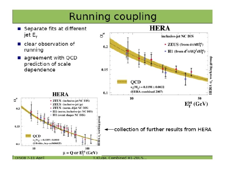
 = 0. 1183 ± 0. 0028 (exp) ±")
Before jets Nice measurement of αs(MZ) = 0. 1183 ± 0. 0028 (exp) ± 0. 0008 (model) From simultaneous fit of αs(MZ) & PDF parameters After jets And correspondingly the contribution of the uncertainty on αs(MZ) to the uncertainty on the PDFs is much reduced And use of jet data can help to tie down both alphas itself and alphas related uncertainties on the gluon PDF

No smoking gun for seomthing new at low-x…so let’s look more exclusively Now let’s look at forward jets Look at the hadron final states. . lack of pt ordering has its consequences. Forward jets with xj » x and ktj 2 ~ Q 2 are suppressed for DGLAP evolution but not for kt disordered BFKL evolution But this has served to highlight the fact that the conventional calculations of jet production were not very well developed. There has been much progress on more sophisticated calculations e. g DISENT, NLOJET, rather than ad-hoc Monte-Carlo calculations (LEPTOMEPS, ARIADNE CDM …) The data do not agree with DGLAP at LO or NLO, or with the Monte-Carlo LEPTO-MEPS. . but agree with ARIADNE is not kt ordered but it is not a rigorous BFKL calculation either………

Forward Jets DISENT vs data NLO below data, especially at small x. Bj but theoretical uncertainty is large Comparison to LO and NLO conventional calculations

Forward Jets Comparison to ARIADNE and LEPTO • Lepto doesn’t suffice • Ariadne default overestimates high Etjet, overestimates high ηjet (proton remnant) • Ariadne tuned is good

SO we started looking at more complex jet production processes…. jet calculations which go up to O(αs 3 ) can describe the dataincluding detailed correlations between x and pt, or x and azimuthal angle
 The negative gluon The corresponding FL")
Q 2 = 2 Ge. V 2 xg(x) The negative gluon The corresponding FL is NOT predicted at low x, low Q 2 negative at Q 2 ~ 2 Ge. V 2 – but from NLO DGLAP remains has peculiar shape at NNLO (worse) Back to considering inclusive quantities Including ln(1/x) resummation in the calculation of the splitting functions (BFKL `inspired’) can improve the shape - and the c 2 of the global fit improves New work in 2007 by White and Thorne

White and Thorne have an NLL BFKL calculation accounting for running coupling AND heavy quark effects – this has various attractive features…… Plus improved χ2 for global PDF fit Other groups working on NLL BFKL are: Ciafaloni, Colferai, Salam, Stasto Altarelli, Ball, Forte But there are no corresponding global fits

Q 2 = 1. 4 Ge. V 2 The use of non-linear evolution equations also improves the shape of the gluon at low x, Q 2 The gluon becomes steeper (high density) and the sea quarks less steep Non-linear effects gg g involve the summation of FAN diagrams – xg xuv xu xd xs xc Non linear DGLAP There is some phenomenology which supports the use of non-linear evolution equations as well, but it is not so well developed Part of our problem is that as well move to low-x we are also moving to lower Q 2 and the non-perturbative region. .

p. QCD region Regge region Linear DGLAP evolution doesn’t work for Q 2 < 1 Ge. V 2, WHAT does? – REGGE ideas? Small x is high W 2, x=Q 2/2 p. q Q 2/W 2 q p px 2 = W 2 (g*p) ~ (W 2) α-1 – Regge prediction for high energy cross-sections α is the intercept of the Regge trajectory α=1. 08 for the SOFT POMERON Such energy dependence is well established from the SLOW RISE of all hadron-hadron cross-sections - including (gp) ~ (W 2) 0. 08 for real photon- proton scattering For virtual photons, at small x (g*p) = 4 2α F 2 Q 2 → ~ (W 2)α-1 → F 2 ~ x 1 -α = x -l so a SOFT POMERON would imply l = 0. 08 gives only a very gentle rise of F 2 at small x For Q 2 > 1 Ge. V 2 we have observed a much stronger rise…. .
 gentle rise QCD improved dipole The slope of F")
much steeper rise F(( *p) gentle rise QCD improved dipole The slope of F 2 at small x , F 2 ~x -l , is equivalent to a rise of (g*p) ~ (W 2)l which is only gentle for Q 2 < 1 Ge. V 2 GBW dipole Regge region p. QCD generated slope So is there a HARD POMERON corresponding to this steep rise? A QCD POMERON, α(Q 2) – 1 = l(Q 2) A BFKL POMERON, α – 1 = l = 0. 5 A mixture of HARD and SOFT Pomerons to explain the transition Q 2 = 0 to high Q 2?

Do we understand the rise of hadron-hadron cross-sections at all? Could there always have been a hard Pomeron- is this why the effective Pomeron intercept is 1. 08 rather than 1. 00? Does the hard Pomeron mix in more strongly at higher energies? What about the at the LHC? Recent work by Caldwell suggests that a double Pomeron model fits best If this is the case in γ*-p, it could be so in p-p But we haven’t noticed yet because the hard Pomeron is not strongly coupled at low energies At the LHC we could notice this But what about the Froissart bound ? – the rise MUST be tamed eventually – non-linear effects/saturation may be necessary Predictions for the p-p cross-section at LHC energies are not so certain

Dipole models provide another way to model the transition Q 2=0 to high Q 2 б(γ*p) The dipole-proton cross section depends on the relative size of the dipole r~1/Q to the separation of gluons in the target R 0 σ =σ0(1 – exp( –r 2/2 R 0(x)2)), R 0(x)2 ~(x/x 0)λ~1/xg(x) r/R 0 small → large Q 2, x σ~ r 2~ 1/Q 2 GBW dipole model Now there is HERA data right across the transition region At low x, γ* → qqbar and the LONG LIVED (qqbar) dipole scatters from the proton But (g*p) = 4 2 F 2 is Q 2 (at small x) r/R 0 large →small Q 2, x general 2 σ ~ σ0 → saturation of (gp) is finite for real photons , Q =0. 2 2 the dipole cross-section At high Q , F 2 ~flat (weak ln. Q breaking) and (g*p) ~ 1/Q 2
) Q 2 > Q")
x < 0. 01 σ = σ0 (1 – exp(-1/τ)) Q 2 > Q 2 s Involves only τ=Q 2 R 02(x), τ= Q 2/Q 02 (x/x 0 )λ Q 2 < Q 2 s And INDEED, for x<0. 01, σ(γ*p) depends only on τ, not on x, Q 2 separately x > 0. 01 τ is a new scaling variable, applicable at small x It can be used to define a `saturation scale’ , Q 2 s = 1/R 02(x). x -λ ~ x g(x), gluon densitysuch that saturation extends to higher Q 2 as x decreases (Qs is low ~1 -2 Ge. V 2 at HERA) Some understanding of this scaling, of saturation and of dipole models is coming from work on non-linear evolution equations applicable at high density– Colour Glass Condensate, JIMWLK, Balitsky-Kovchegov. There can be very significant consequences for high energy cross-sections (LHC and neutrino), predictions for heavy ions- RHIC, diffractive interactions etc.

The Pomeron also makes less indirect appearances in HERA data in diffractive events, which comprise ~10% of the total. The proton stays more or less intact, and a Pomeron, with fraction XP of the proton’s momentum, is hit by the exchanged boson. One can picture partons within the Pomeron, having fraction β of the Pomeron momentum One can define diffractive structure functions, which broadly factorize in to a Pomeron flux (function of x. P, t) and a Pomeron structure function (function of β, Q 2). The Pomeron flux has been used to measure Pomeron Regge intercept – which come out marginally harder than that of the soft Pomeron The Pomeron structure functions indicate a large component of hard gluons in the Pomeron

But this is not the only view of difraction. These data have also been interpretted in terms of dipole models If the total cross-section is given by σ ~∫ d 2 r dz (׀ ψ(z, r) ׀ 2 σdipole(W) Then the diffractive cross-section can be written as σ ~ ∫ d 2 r dz (׀ ψ(z, r) ׀ 2 σdipole 2(W) The fact that the ratio of σdiff/σtot is observed to be constant implies a constant σdipole which could indicate saturation Colour. Dipole. Model fits to ZEUS diffractive data

Ther is more evidence for hard Pomeron behaviour from diffractive Vector meson production and DVCS These processes are ~elastic γ*p → V p Hence if σtot ~Im Aelastic ~ W 2(α 0)-1) Then σelastic ~ ׀ Aelastic ׀ 2 ~ W 4(α(0)-1) A soft Pomeron α(0)~1. 08 would give σelastic ~ W 0. 32 A hard Pomeron α(0)~1. 3 would give σ elastic ~ W 1. 2 The experimental measurements vary from soft to hard depending on whethere is a hard scale in the process We can plot the effective Pomeron intercepts vs Q 2+MV 2 DVCS also seems to show a form of geometric scaling

Summary What have we learnt from DIS in the last 30 -35 years? • Verified the basic idea of QPM • Established QCD as theory of the strong interaction • Measurement of essential parameters: Parton Distribution Functions, αs(MZ ) and the running of αs • Low-x physics • QCD beyond DGLAP. . BFKL. . non-linear. . CGC. . dipole models. . diffraction etc • The LHC could discover a different kind of new physics
- Slides: 76