Decomposition of the Total Effect into Substitution and

Decomposition of the Total Effect into Substitution and Income Effects Week 4

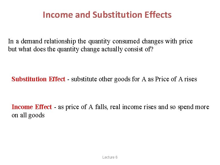
Income and Substitution Effects In a demand relationship the quantity consumed changes with price but what does the quantity change actually consist of? Substitution Effect - substitute other goods for A as Price of A rises Income Effect - as price of A falls, real income rises and so spend more on all goods Lecture 6

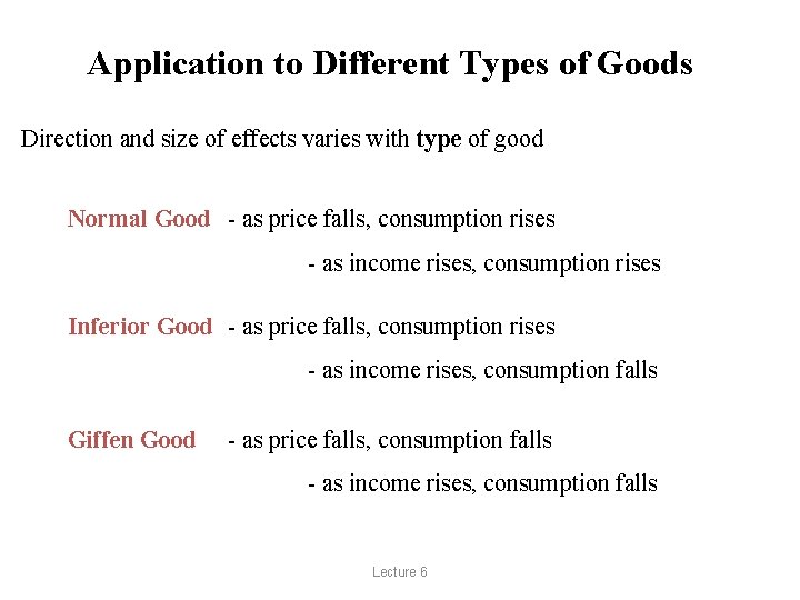
Application to Different Types of Goods Direction and size of effects varies with type of good Normal Good - as price falls, consumption rises - as income rises, consumption rises Inferior Good - as price falls, consumption rises - as income rises, consumption falls Giffen Good - as price falls, consumption falls - as income rises, consumption falls Lecture 6

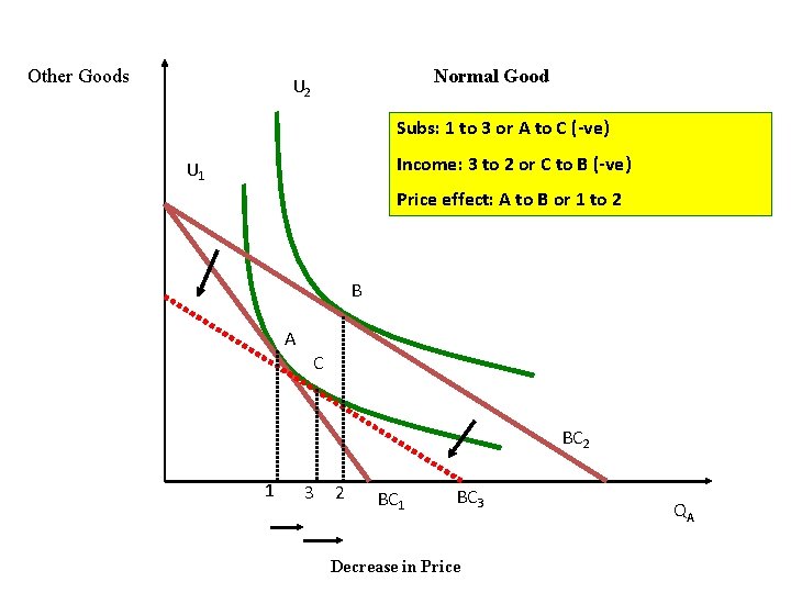
Other Goods Normal Good U 2 Subs: 1 to 3 or A to C (-ve) Income: 3 to 2 or C to B (-ve) U 1 Price effect: A to B or 1 to 2 B A C BC 2 1 3 2 BC 1 BC 3 Decrease in Price QA

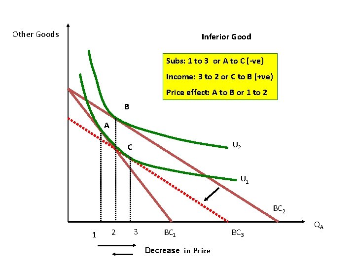
Other Goods Inferior Good Subs: 1 to 3 or A to C (-ve) Income: 3 to 2 or C to B (+ve) Price effect: A to B or 1 to 2 B A U 2 C U 1 BC 2 1 2 3 BC 1 Decrease in Price BC 3 QA

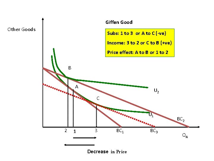
Giffen Good Other Goods Subs: 1 to 3 or A to C (-ve) Income: 3 to 2 or C to B (+ve) Price effect: A to B or 1 to 2 B A U 2 C U 1 2 1 3 BC 1 Decrease in Price BC 3 BC 2 QA

Income and Substitution Effects • Slutsky equation • Total effect of price change = SE + IE • Slutsky’s theorem states that the substitution effect of a price change (relative to quantity) is negative. • We isolate the substitution effect by taking away from (giving) the consumer enough money to put her at the same level of satisfaction as before the price change. 7

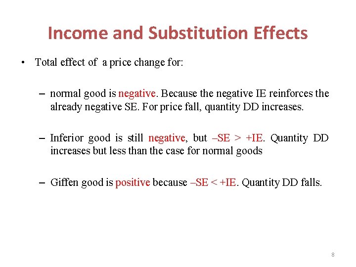
Income and Substitution Effects • Total effect of a price change for: – normal good is negative. Because the negative IE reinforces the already negative SE. For price fall, quantity DD increases. – Inferior good is still negative, but –SE > +IE. Quantity DD increases but less than the case for normal goods – Giffen good is positive because –SE < +IE. Quantity DD falls. 8

Labor-Leisure Choice • Leisure - all time spent not working. • The number of hours worked per day, H, equals 24 minus the hours of leisure or nonwork, N, in a day: H = 24 − N. – The price of leisure is forgone earnings. • The higher your wage, the more an hour of leisure costs you.

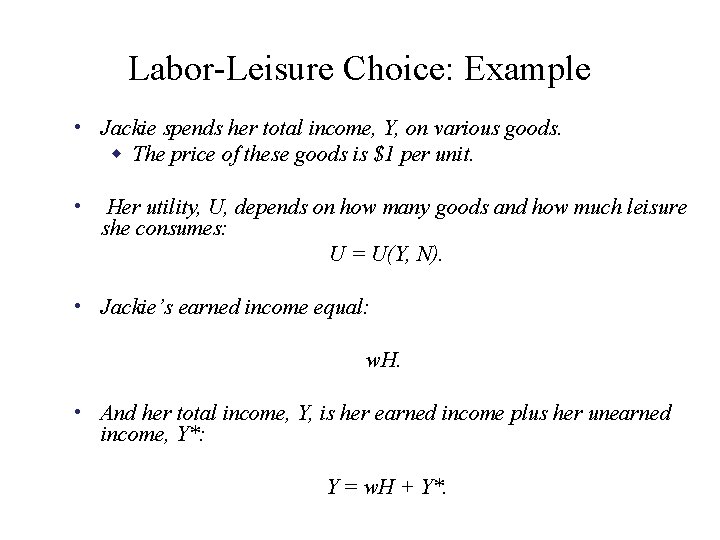
Labor-Leisure Choice: Example • Jackie spends her total income, Y, on various goods. w The price of these goods is $1 per unit. • Her utility, U, depends on how many goods and how much leisure she consumes: U = U(Y, N). • Jackie’s earned income equal: w. H. • And her total income, Y, is her earned income plus her unearned income, Y*: Y = w. H + Y*.

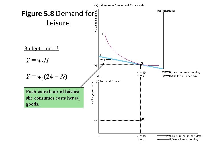
(a) Indifference Curves and Constraints Figure 5. 8 Demand for Leisure Y , Goods per day Time constraint I 1 Budget Line, L 1 –w 1 Y = w 1 H 0 24 w, Wage per hour Y = w 1(24 − N). Each extra hour of leisure she consumes costs her w 1 goods. 1 Y 1 e 1 N 1 = 16 H 1 = 8 24 0 N, Leisure hours per day H, Work hours per day (b) Demand Curve E 1 w 1 0 N 1 = 16 H 1 = 8 N, Leisure hours per day H, Work hours per day

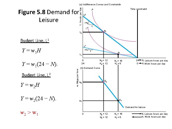
Y, Goods per day (a) Indifference Curves and Constraints Figure 5. 8 Demand for Leisure Time constraint I 2 L 2 –w 2 1 I 1 e 2 Y 2 Budget Line, L 1 –w 1 Y = w 1 H 0 24 Y = w 2 H Y = w 2(24 − N). w, Wage per hour Y = w 1(24 − N). Budget Line, L 2 1 e 1 Y 1 N 2 = 12 H 2 = 12 N 1 = 16 H 1 = 8 24 0 N, Leisure hours per day H, Work hours per day (b) Demand Curve E 2 w 2 E 1 w 1 Demand for leisure w 2 > w 1 0 N 2 = 12 H 2 = 12 N 1 = 16 H 1 = 8 N, Leisure hours per day H, Work hours per day

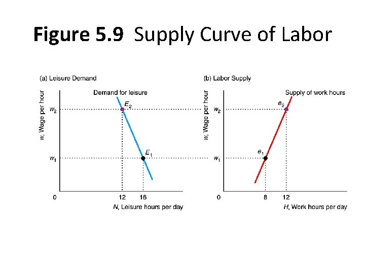
Figure 5. 9 Supply Curve of Labor

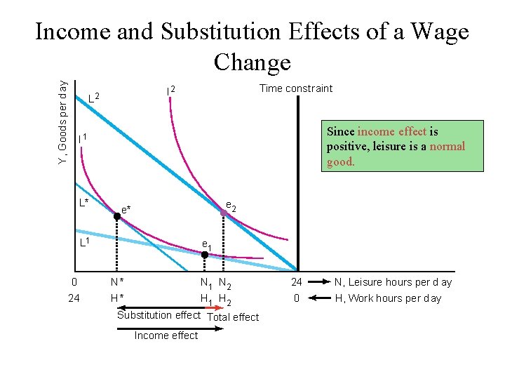
Y, Goods per d ay Income and Substitution Effects of a Wage Change Time constraint I 2 L 2 Since income effect is positive, leisure is a normal good. I 1 L* e 2 e* L 1 e 1 0 N* N 1 N 2 24 N, Leisure hours per d ay 24 H* H 1 H 2 0 H, Work hours per d ay Substitution effect Total effect Income effect

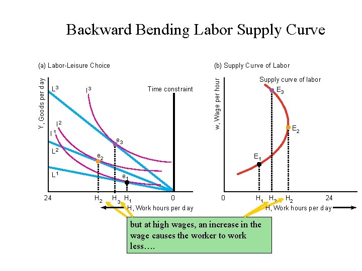
Backward Bending Labor Supply Curve L 3 (b) Supply Curve of Labor Time const raint I 3 I 2 I 1 L 2 E 3 E 2 e 3 e 2 E 1 L 1 24 Supply curve of labor w, Wage per hour Y, Goods per d ay (a) Labor-Leisure Choice e 1 H 2 H 3 H 1 0 0 H 1 H 3 H, Work hours per d ay butlow At at high wages, an increase in the wage causes the worker to work more…. less…. H 2 24 H, Work hours per d ay

Ordinary curve vrs compensated demand curve • Compensating variation ensures that the consumer remains on the same IC. DDc is steeper than ordinary DDo curve. The slope of the DDc curve is larger for a normal good. The Hicksian demand function. • Ordinary DDo curve considers the effect of IE. The DDo is flatter. The slope of the DDo curve is smaller. The Marshallian demand function. • The Marshallian demand function is the ordinary market demand function we have been discussing all along. 16

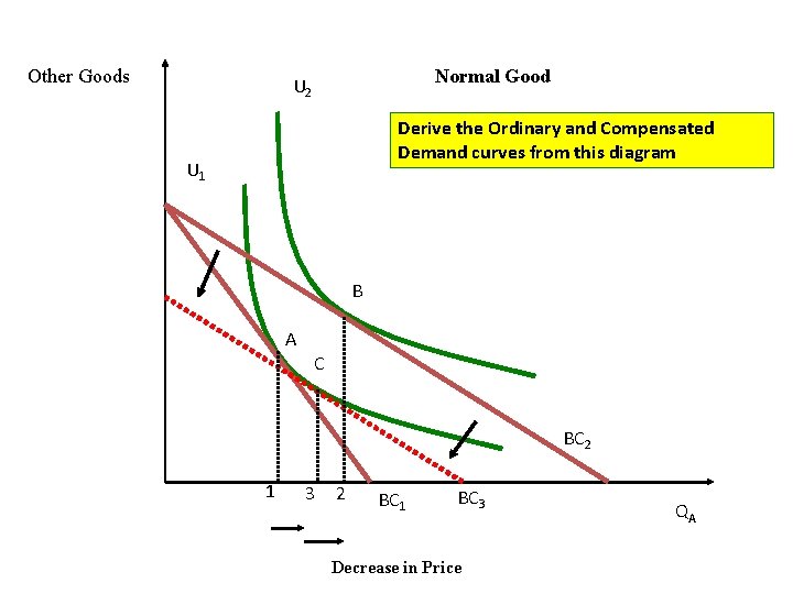
Other Goods Normal Good U 2 Derive the Ordinary and Compensated Demand curves from this diagram U 1 B A C BC 2 1 3 2 BC 1 BC 3 Decrease in Price QA

End