Decomposition Methods Overview of two of the main

Decomposition Methods

Overview of two of the main decomposition methods used – To solve large scale problem – To take advantage of structures embedded in the problem

Problem types Min f (x) Subject to x ε X 1 x ε X 2 Min f (x, y) Subject to F (x, y) ≤ 0 x ε X, y ε Y X 1: nice constraints X 2: annoying constraints x : nice variables y : annoying variables Column generation (Dantzig – Wolfe Decomposition) Constraint generation (Benders Decomposition)

Presentation • Illustrate with linear constraints but the methods can be generalized.

COLUMN GENERATION (DANTZIG – WOLFE DECOMPOSITION)

Problem formulation Min f (x) Subject to x ε X 1 x ε X 2 X 1: nice constraints X 2: annoying constraints Min c. Tx Subject to Ax=b xεX

Property of the nice constraints X polyedral convex set: Min c. Tx Subject to Ax=b xεX λi ≥ 0 1≤i≤r

Property of the nice constraints Min c. Tx Subject to Ax=b xεX

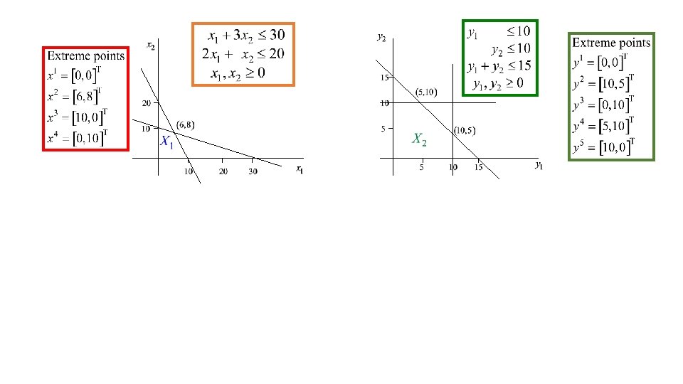
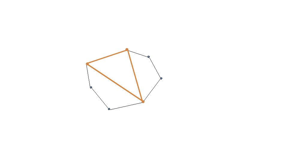
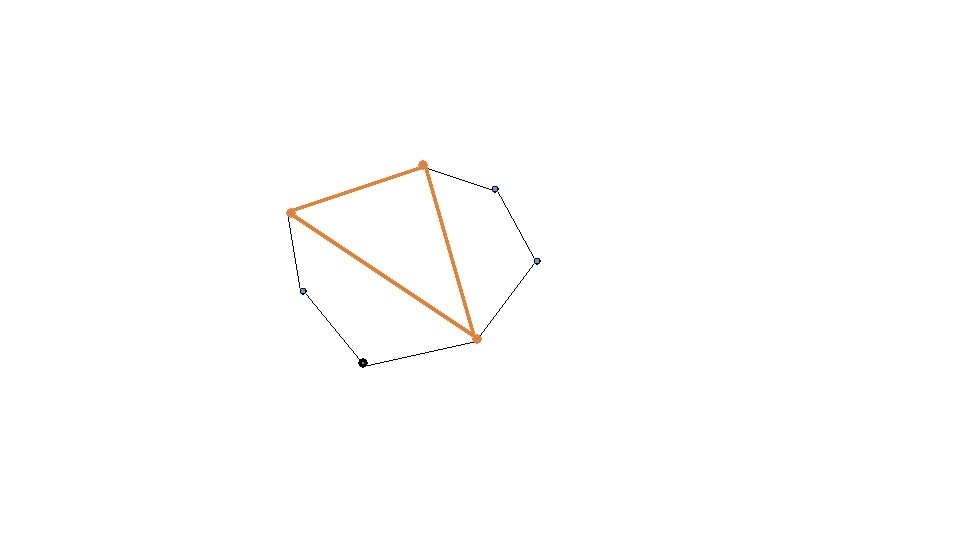
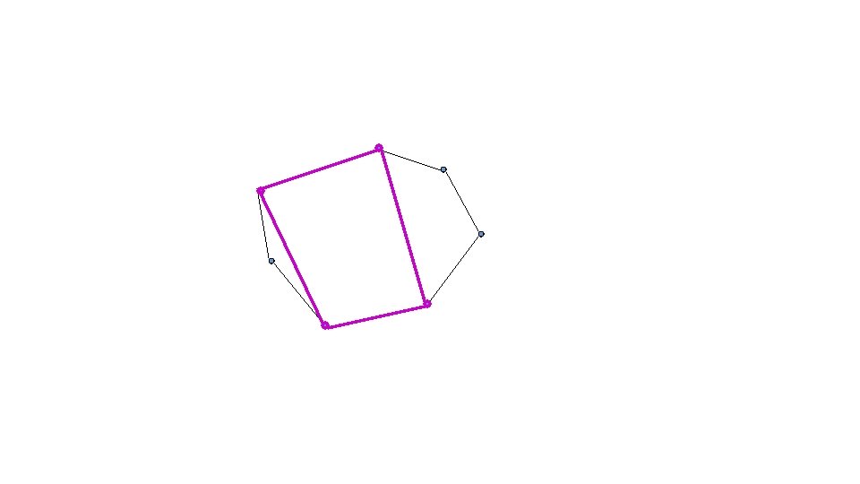
Property of the nice constraints X polyedral convex set: Min c. Tx Subject to Ax=b xεX Set of extreme points of X: {x 1, x 2, …, xr} x ε X <=> x = ∑ 1≤i≤r λi xi ∑ 1≤i≤r λi = 1 λi ≥ 0 1≤i≤r

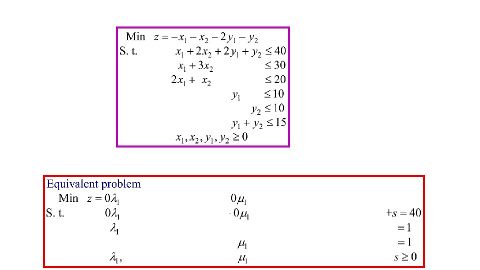
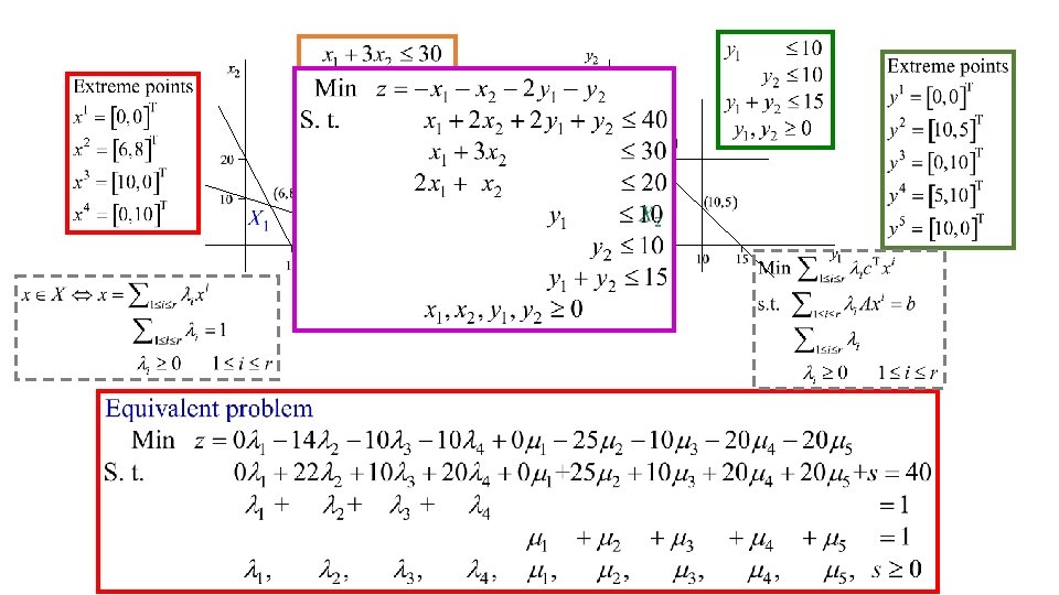
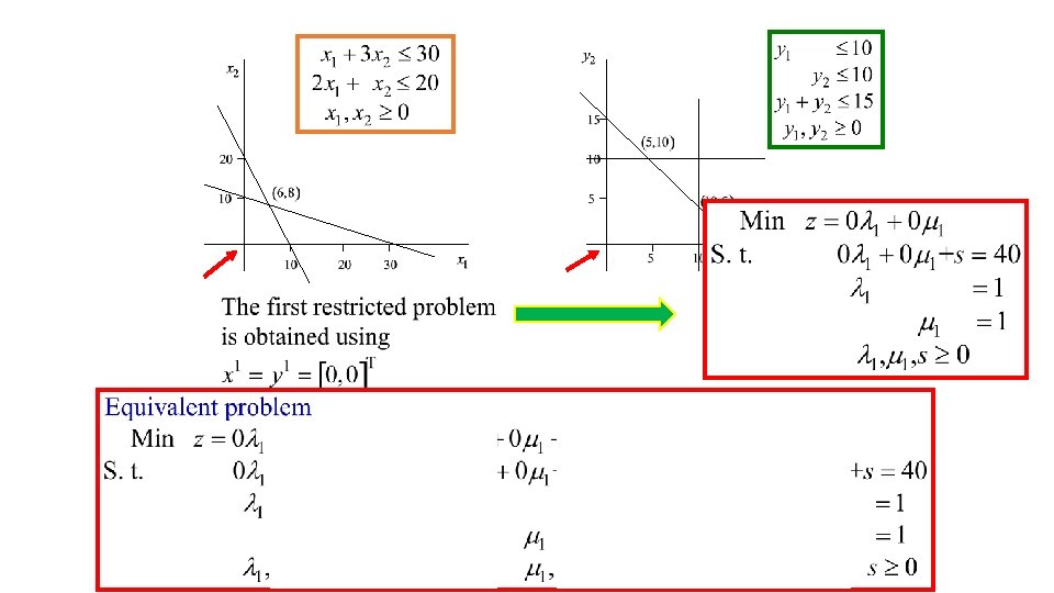
Numerical example

Equivalent problem Min c. Tx Subject to Ax=b xεX Min ∑ 1≤i≤r λi c. Txi Subject to ∑ 1≤i≤r λi A xi = b ∑ 1≤i≤r λi = 1 λi ≥ 0 1≤i≤r X polyedral convex set Set of extreme points of X: {x 1, x 2, …, xr} x ε X <=> x = ∑ 1≤i≤r λi xi ∑ 1≤i≤r λi = 1 λi ≥ 0 1≤i≤r

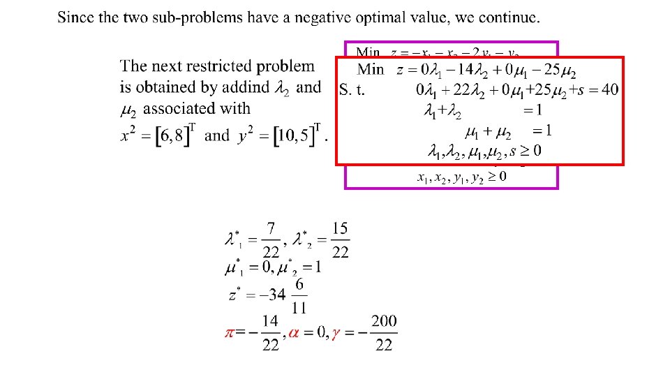
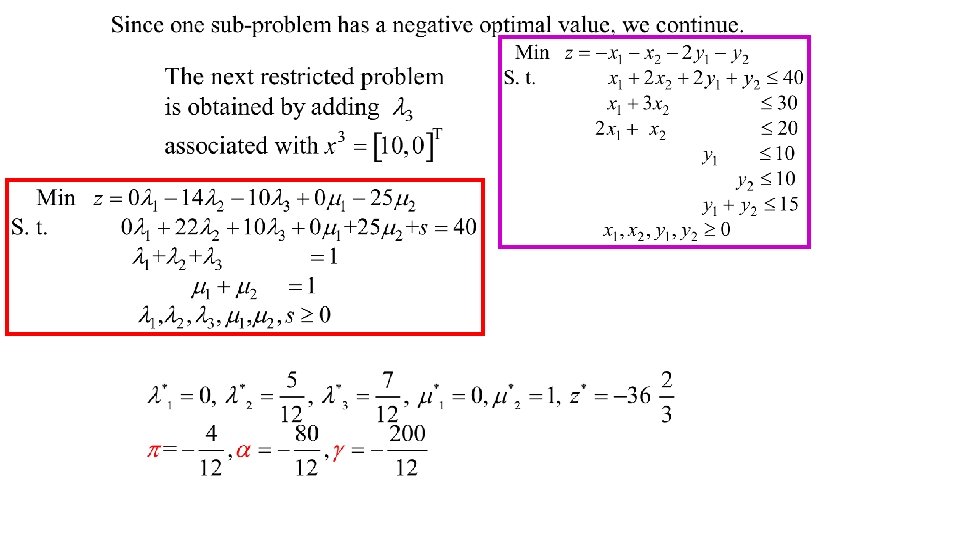
Solution approach Solve a sequence of restricted problems (λi = 0 as long as xi is not generated) Min ∑iεG λi c. Txi Subject to ∑iεG λi A xi = b ∑iεG λi = 1 λi ≥ 0 iεG where G = {i: xi is already generated}

Column generation Mechanism 1. to verify if the optimal solution λi*, iεG, of a restricted problem is optimal for the problem or if not, 2. to generate additional variables to be added in order to define a new restricted problem

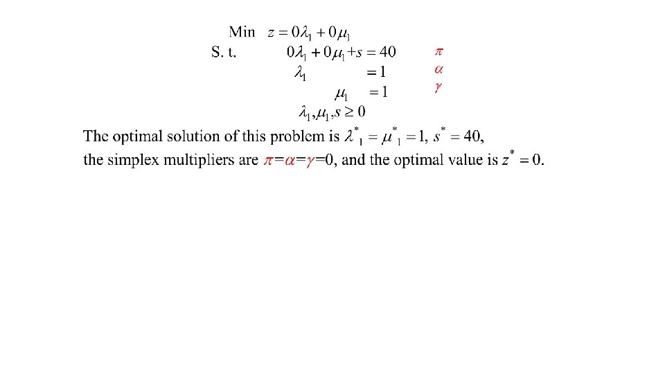
Solve the restricted problem Min ∑iεG λi c. Txi Subject to ∑iεG λi A xi = b ∑iεG λi = 1 λi ≥ 0 Let iε G λi*, iε G be an optimal solution

Price out the variables Relative costs of the variables λi i εG Min ∑iεG λi c. Txi Subject to c. T xi – πT A x i – α ≥ 0 ∑iεG λi A xi = b π ∑iεG λi = 1 α λi ≥ 0 Let i εG λi*, i εG be an optimal solution Simplex multipliers

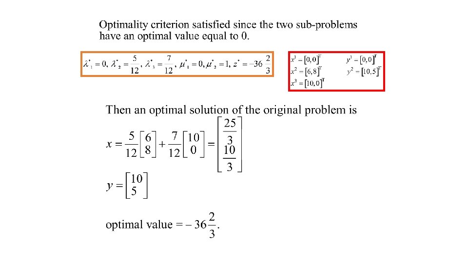
Checking optimality Min ∑ 1≤i≤r λi c. Txi Subject to ∑ 1≤i≤r λi A xi = b ∑ 1≤i≤r λi = 1 λi ≥ 0 1≤i≤r Then x* = ∑ iεG λi* xi is an optimal solution of the original problem Relative cost of the variables λi i εG c Tx i – π TA x i – α ≥ 0 The solution λi = λi*, i εG λi = 0 i εG is optimal for the equivalent problem if c. Txi – πTA xi – α ≥ 0 1≤i≤r

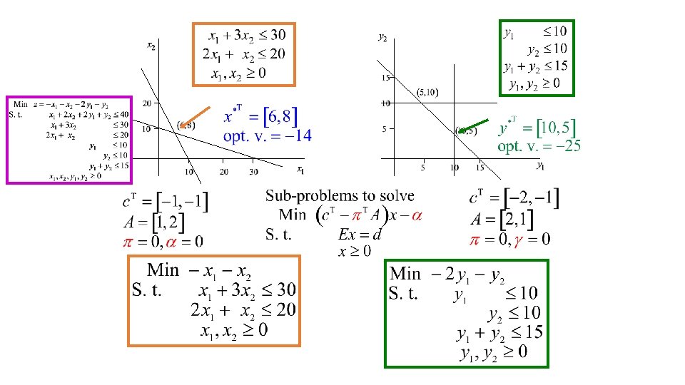
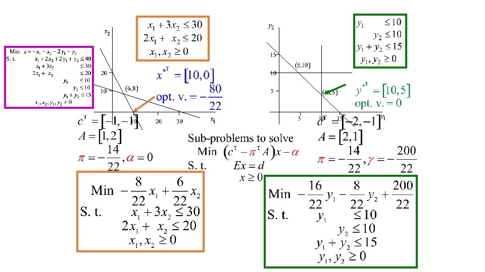
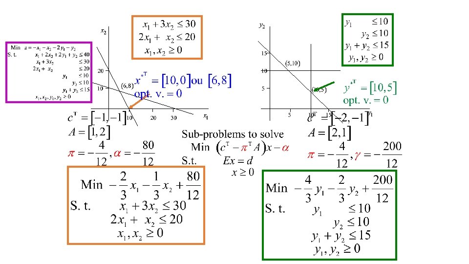
Solving a problem with the nice constraints Relative costs of the variables λi i εG c. T xi – πT A x i – α ≥ 0 The solution λi = λi*, i εG λi = 0 i εG is optimal for the equivalent problem if c. Txi – πTA xi – α ≥ 0 1≤i≤r <=> Min 1≤i≤r {c. Txi – πTA xi – α } ≥ 0 <=> Minx ε X {c. Tx – πTA x – α } ≥ 0 • Hence verify if the optimal value of Min c. Tx – πTA x – α Subject to xε is ≥ 0

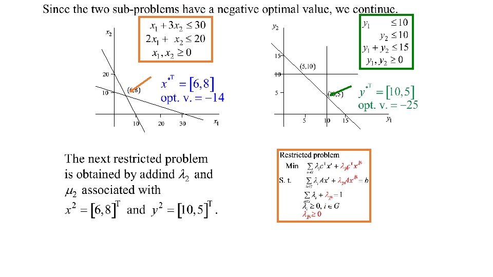
Column generation Hence if the optimal value of Min c. Tx – πTA x – α Subject to xε is ≥ 0 Otherwise, if c. Txμ – πTA xμ – α = Minx ε X {c. Tx – πTA x – α } < 0, then xμ ε {x 1, x 2, …, xr}. The associated variable Then x* = ∑ iεG λi* xi is an optimal solution of the original problem λμ has a negative relative cost and is included to generate a new restricted problem

New restricted problem Min ∑iεG λi c. Txi + λμ c. Txμ Subject to ∑iεG λi A xi + λμ A xμ = b ∑iεG λi + λμ = 1 λi ≥ 0 λμ ≥ 0 iεG Otherwise, if c. Txμ – πTA xμ – α = Minx ε X {c. Tx – πTA x – α } < 0, then xμ ε {x 1, x 2, …, xr}. The associated variable λμ has a negative relative cost and is included to generate a new restricted problem

Hence if the optimal value of Min c. Tx – πTA x – α Subject to xε is ≥ 0 Otherwise, if c. Txμ – πTA xμ – α = Minx ε X {c. Tx – πTA x – α } < 0, then xμ ε {x 1, x 2, …, xr}. The associated variable Then x* = ∑ iεG λi* xi is an optimal solution of the original problem λμ has a negative relative cost and is included to generate a new restricted problem

Convergence of the restriction approach Convergence of the method D-W method completed in a finite number of iterations: The set of extreme points {x 1, x 2, …, xr} of X is finite At each iteration of the D-W method, at least one new variable λμ associated with one extreme point xμ ε {x 1, x 2, …, xr} is added to generate a new restricted problem.

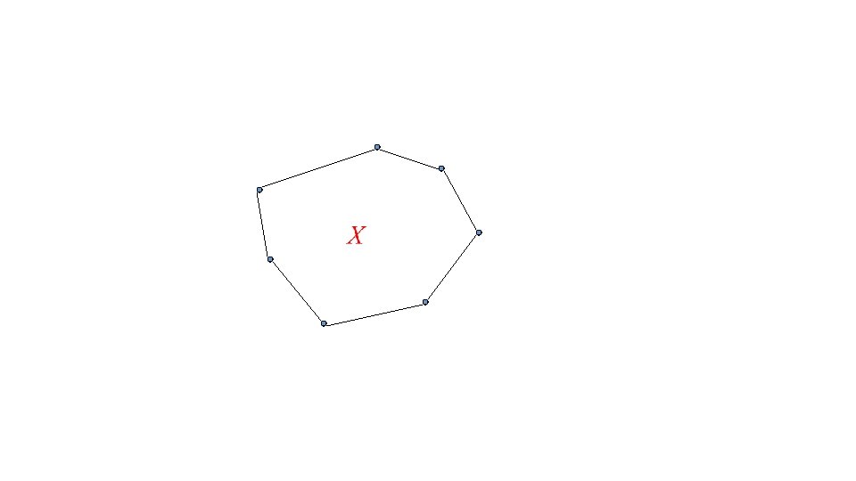
X

Advantages • Solve a sequence of restricted (smaller) problems • Mechanism to verify if the optimal solution of restricted problem is optimal for the original problem: solving a problem specified with the nice constraints • Same mechanism generates additional variables to modify the restricted problem and to get closer to the original one

Advantage of the approach • PRIMAL METHOD: for any restricted problem the optimal solution λi*, iεG x = ∑ iεG λi* xi feasible for the original problem

Extensions • X polyedron (unbounded) convex. • Generate the initial set of extreme points G using some kind of phase I of the simplex. • X convex set.