Declining inequality in Latin America a decade of

Declining inequality in Latin America: a decade of progress? Eds. Lopez-Calva and Lustig (Brookings Institution Press and UNDP, 2010) Nora Lustig Samuel Z. Stone Professor of Latin American Economics Dept. of Economics Tulane University Nonresident Fellow, Center for Global Development and Inter-American Dialogue Meeting of Western Hemisphere Think Tanks in Support of the Summit of the Americas Bogotá, March 14, 2011 1

Latin America is the most unequal region in the world Using Gini coefficient, 19 percent more unequal than Sub-Saharan Africa 37 percent more unequal than East Asia 65 percent more unequal than developed countries 2

Gini Coefficient by Region (in %), 2004 3

Gini Coefficient for Latin America: early 1990 s-mid 2000 s (Gasparini et al. , 2009) 5

Declining Inequality in LA Inequality in most Latin American countries (12 out of 17) has declined (roughly 1. 1% a year) between (circa) 2000 and (circa) 2007. Except in two cases, decline is statistically significant. (rectangles in grey in next slide) 6

Change in Gini Coefficient by Country: circa 2000 -2007 (yearly change in percent) 1. 50 1. 00 0. 79 0. 89 0. 98 1. 02 0. 50 0. 05 0. 00 -0. 24 -0. 36 -0. 29 -0. 50 -0. 37 -0. 56 -1. 00 -1. 50 -1. 40 -1. 27 -1. 12 -1. 00 -0. 99 -0. 83 -0. 88 -0. 83 Total 17 countries Total 12 countries Nicaragua Costa Rica Uruguay Honduras Guatemala Venezuela Ecuador Bolivia Panama Paraguay Peru Dominican Rep. Argentina Chile Brazil Mexico El Salvador -2. 00 7

8

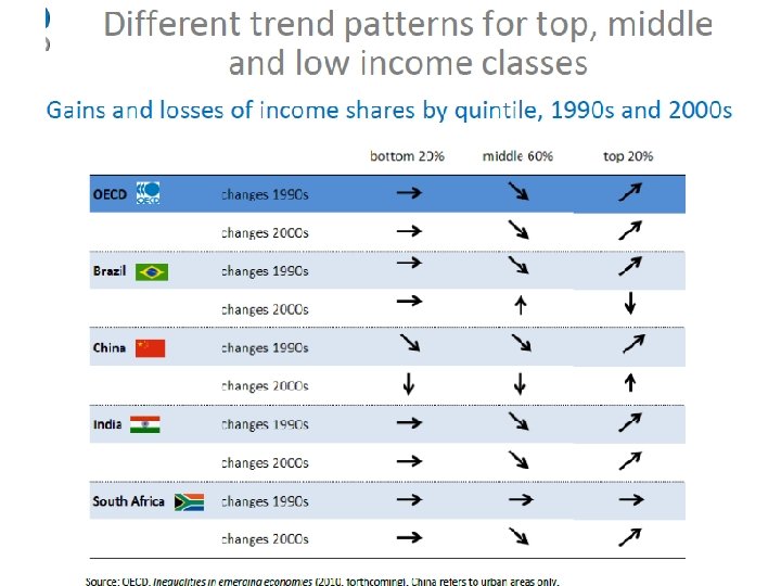
The decline in inequality has been widespread The decline took place in: Persistently high inequality countries (Brazil) and normally low inequality countries (Argentina) Fast growing countries (Chile and Peru), slow growing countries (Brazil and Mexico) and countries recovering from crisis (Argentina and Venezuela) Countries with left populist governments (Argentina), left social-democratic governments (e. g. , Brazil, Chile) and centerright governments (e. g. , Mexico and Peru) 10

Main Questions: Why has inequality declined in Latin America? Are there factors in common? In-depth analysis in four countries: Argentina (Gasparini and Cruces) (urban; 2/3 of pop) Brazil (Barros, Carvalho, Mendoca & Franco) Mexico (Esquivel, Lustig and Scott) Peru (Jaramillo & Saavedra) 11

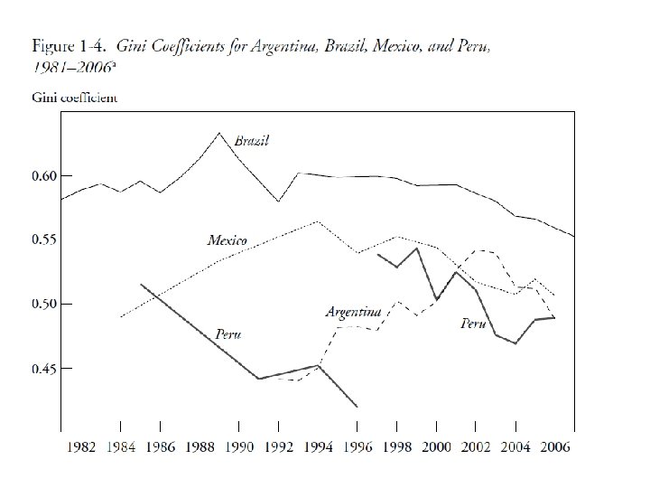
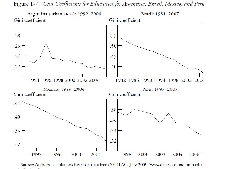
Inequality has continued to decline in Brazil The Gini Coefficient reached its lowest level in the last three decades. 1981 -2009

Argentina (urban areas): 1992 -2009 (Gasparini, 2010)

Decline is robust Decline in inequality is statistically significant and significant in terms of order of magnitude There is Lorenz dominance (unambiguous decline independently of choice of inequality measure) Robust to income concept (e. g. , monetary vs. total) 16

Four countries are a. . . Representative sample of Latin American diversity: high/medium/low ineq high/low growth Populist/social democratic/centerright governments 17

Sample Representative of High and Low Inequality Countries (Latin America: Gini Coefficient by Country; circa 2007; in percent) 18

Sample Representative of High and Low Growth Countries

Argentina: Growth Incidence Curves 20

Brazil: GICs 2001 -06 21

Over the last years, the income of the Brazilian poor has been growing as faster as per capita GDP in China. By the other hand, the income of the richest has been growing as faster as per capita GDP in Germany.

Mexico: GICs 2000 -06 23

Peru: GICs 1997 -2006 24

Are results credible?

Proximate and fundamental determinants of changes in inequality There are many different factors that affect the distribution of income over time: “… the evolution of the distribution of income is the result of many different effects—some of them quite large—which may offset one another in whole or in part. ” (Bourguignon et al. , 2005) Useful framework: to consider the ‘proximate’ factors that affect the distribution of income at the individual and household level: 1. 2. 3. 4. 5. Distribution of assets and personal characteristics Return to assets and characteristics Utilization of assets and characteristics Transfers (private and public) Socio-demographic factors 29

Four countries share two relevant socio-demographic changes Proportion of working adults as a share of the total number of adults (and total household members) rose; partly linked to the sharp increase in female labor force participation: 1990 -2006 by 18. 1 p. pts in Mexico, 14. 2 in Argentina, 12. 0 in Brazil and 5. 8 in Peru. ÞDependency ratios improved proportionately more for low incomes. ÞWorking adults (except for Peru) became more equally distributed (female adults participated proportionately more for low incomes) Average years of schooling rose faster for the bottom quintile than for the top quintile. => Distribution of education (human capital) became more equal in all four countries 30

31

Household per capita income and its determinants Per capita household income DEMOGRAPHIC Proportion of adults in the household • FERTILITY • MARKET • POLITICS/ INST. • STATE • DEMOGRAPHIC • MARKET Household income per adult Household non-labor income per adult • RENTS & PROFITS • REMITTANCES • GOV. TRANSFFERS Household labor income per adult Proportion of working adults • PARTICIPATION IN LABOR FORCE • EMPLOYMENT OPPORT • DEMOGRAPHIC • MARKET • POLITICS/INST. / SOC. NORMS • STATE (EDUCATION) Labor income per working adult in the household • WAGES BY SKILL/OTHER • HOURS WORKED 32

Decomposing changes into proximate determinants (Barros et al. 2006, 2007) Per capita household income can be written as: y = a ( u w + o) This identity relates changes in per capita household income, y, to its four proximate determinants: changes in the proportion of adults in the household, a; (ii) changes in the proportion of working adults, u; (iii) changes in labor income per working adult in the household, w; and (iv) changes in household non-labor income per adult, o. (i) 33

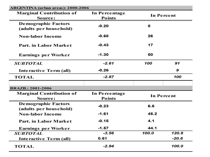
Decomposition results (Alejo et al. , 2009): Demographics: Changes in the ratio of adults per household were equalizing, albeit the orders of magnitude were generally smaller except for Peru. Labor force participation: With the exception of Peru, changes in labor force participation (the proportion of working adults) were equalizing. This effect was stronger in Argentina. 36

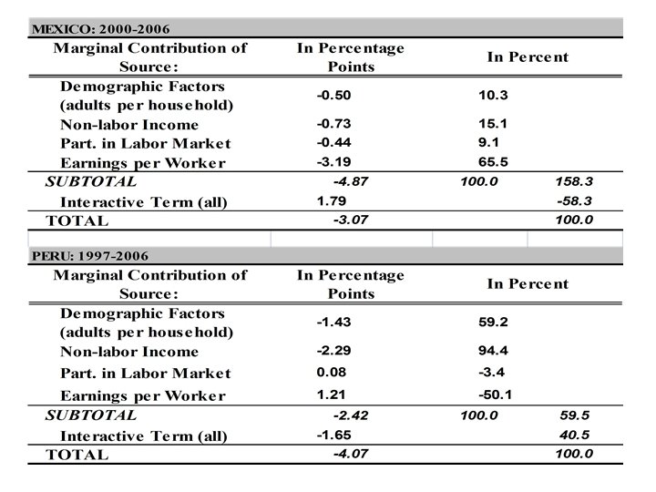
Decomposition results (Alejo et al. , 2009): Labor income (Earnings): In Argentina, Brazil, and Mexico between 44% and 65% of the decline in overall inequality is due to a reduction in earnings per working adult inequality. In Peru, however, changes in earnings inequality were unequalizing at the household level but not so at the individual workers’ level. Non-labor income: Changes in the distribution of non-labor income were equalizing; the contribution of this factor was quite high in Brazil and Peru (45% and 90%, respectively). 37

Decomposition results (Alejo et al. , 2009): => Decline in labor inc 0 me (except for Peru at the household level) and non-labor income inequality important determinants of the decline in overall income inequality (in per capita household income) 38

Argentina: 2004 -06 (Gasparini & Cruces) Decline in labor income inequality: employment generated by recovery: open unemployment fell from 14. 8% in 2000 to 9. 6% in 2006 shift in favor of more low-skilled, labor-intensive sectors as a result of the devaluation rise in the influence of labor unions which compresses wages fading of the one-time effect of skill-biased technical change that occurred in the 1990 s Decline in non-labor income inequality: more progressive government transfers: Jefes y Jefas de Hogar program launched in 2002 39

40

Argentina: Distributional impact of Conditional cash transfers 41

Brazil: 2001 -2007 (Barros et al. ) Decline in labor income inequality: About 50% accounted for by decline in attainment inequality (quantity effect) and less steep returns -wage gap by skill narrows—(price effect). Latter dominant. (See Gini for years of schooling and returns by skill in next two slides) About 25% accounted for by decline in spatial segmentation; especially, reduction in wage differentials between metropolitan areas and medium/small municipalities. Also, decline in sectoral segmentation. 42

43

45

Decline in non-labor income inequality Contribution of changes in the distribution of income from assets (rents, interest and dividends) and private transfers was unequalizing but limited. Most of the impact of non-labor income on the reduction of overall income inequality was due to changes in the distribution of public transfers: changes in size, coverage and distribution of public transfers. Bolsa Familia accounts for close to 10 percent of the decline in household per capita income inequality. 46

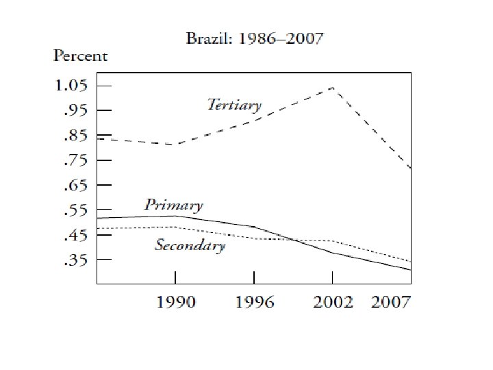
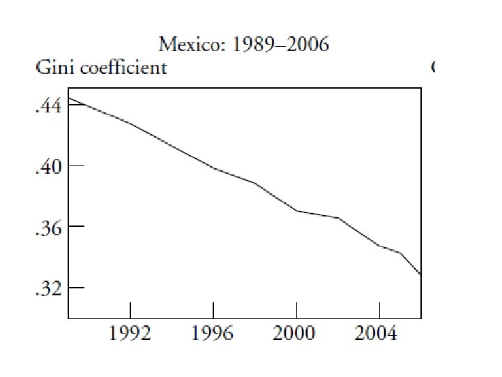
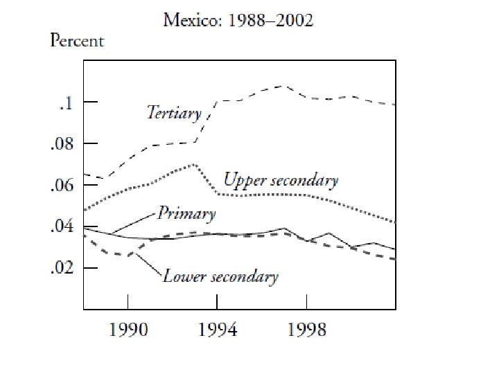
Mexico: 2000 -2006 (Esquivel, Lustig & Scott, 2009) Decline in labor income inequality: Educational attainment became more equal and returns less steep. The latter seems to be associated with the decline in relative supply of workers with low educational levels. Between 1989 and 2006, the share of workers with less than lower-secondary education fell from 55% to around 33%. It coincides with the period in which government gave a big push to basic education. ▪ Between 1992 and 2002 spending per student in tertiary education expanded in real terms by 7. 5 percent while it rose by 63 percent for primary education. ▪ The relative ratio of spending per student in tertiary vs. primary education thus declined from a historical maximum of 12 in 1983 -1988, to less than 6 in 19942000 (by comparison, the average ratio for high-income OECD countries is close to 2). Next two slides show: Gini for yrs. of schooling and returns to schooling 47

Decline in non-labor income inequality The equalizing contribution of government transfers increased over time (both at the national level as well as for urban and, especially, rural households). By 2006 transfers became the income source with the largest equalizing effect of all the income sources considered. Remittances became more equalizing too but with a smaller effect than government transfers. Both more than offset the increasingly unequalizing impact of pensions. 50

Decline in non-labor income inequality The sharp rise in the role and equalizing impact of public transfers was a consequence of a significant policy shift in 1997, when the government launched the conditional cash transfer program Progresa/Oportunidades. During 1996 -2006 the size of public transfers increased; they became more equally distributed among recipients, and the recipients of transfers increasingly belonged to relatively poorer segments of the population. 51

52

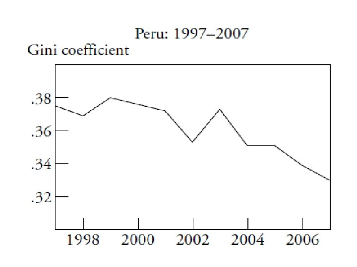
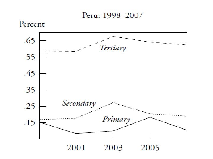
Peru: 1997 -2006 (Jaramillo & Saavedra, 2009) Labor income inequality: Changes in educational structure were equalizing at the household and individual workers levels. Changes in returns to education, however, were equalizing at the individual workers level but not at the household level. Changes in assortative matching might have been a factor. Earnings gap by skill narrowed at the individual workers level as in the other countries. Fading out of skill-biased technical change and a more equal distribution of education/educational upgrading. Next two slides show the Gini for years of schooling and the returns to schooling. 53

Decline in non-labor income inequality: progressivity rose in nonmonetary transfers 56

Why has inequality declined? Main findings Educational upgrading and a more equal distribution of educational attainment have been equalizing (quantity effect). No “paradox of progress” this time. Changes in the steepness of the returns to education curve have been equalizing at the individual workers level (price effect). Except for Peru, they have been equalizing at the household level too. Changes in government transfers were equalizing: more progressive government transfers (monetary and in-kind transfers); expansion of coverage, increase in the amount of transfers per capita, better targeting. 57

59

Why has the skill premium declined? Increase in relative demand for skilled labor petered out: Fading of the unequalizing effect of skill-biased technical change in the 1990 s: Argentina, Mexico & Peru. Decline in relative supply of low-skilled workers: Expansion of basic education since the 1990 s: Brazil, Mexico and Peru. 61

62

Why has earnings inequality declined? Other effects: Decline in spatial labor market segmentation in Brazil. In the case of Argentina, the decline also driven by a pro-union government stance and by the impetus to low-skill intensive sectors from devaluation. In Brazil, increase in minimum wages. 64

Why has inequality in non-labor incomes declined? In the four countries government transfers to the poor rose and public spending became more progressive ▪ In Argentina, the safety net program Jefes y Jefas de Hogar. ▪ In Brazil and Mexico, large-scale conditional cash transfers => can account for between 10 and 20 percent of reduction in overall inequality. An effective redistributive machine because they cost around. 5% of GDP. ▪ In Peru, in-kind transfers for food programs and health. Also access to basic infrastructure for the poor rose. 65

Conclusions In the race between skill-biased technological change and educational upgrading, in the last ten years the latter has taken the lead (Tinbergen’s hypothesis) Perhaps as a consequence of democratization and political competition, government (cash and inkind) transfers have become more generous and targeted to the poor Will the momentum towards a less unequal Latin America continue? 66

Is Inequality Likely to Continue to Fall? Despite the observed progress, inequality continues to be very high and the bulk of government spending is not progressive. The decline in inequality resulting from the educational upgrade of the population will eventually hit the ‘access to tertiary education barrier’ which is much more difficult to overcome: inequality in quality and ‘opportunity cost’ are high and costly to address. Making public spending more progressive in the future is likely to face more political resistance (entitlements of some powerful groups). 67

THANK YOU 68

Appendix: socio-economic indicators 69

Appendix: Income concept Argentina: current monetary (no imputations for owner’s occupied housing); assumes it’s after taxes for wage earners & before for other (assumption); after monetary government transfers (in survey). Brazil: current monetary plus imputed value of income in kind (no imputations for owner’s occupied housing); before taxes (assumption) and after monetary government transfers (in survey and assumption). 70

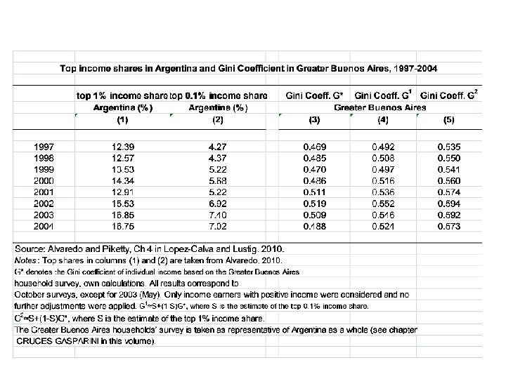
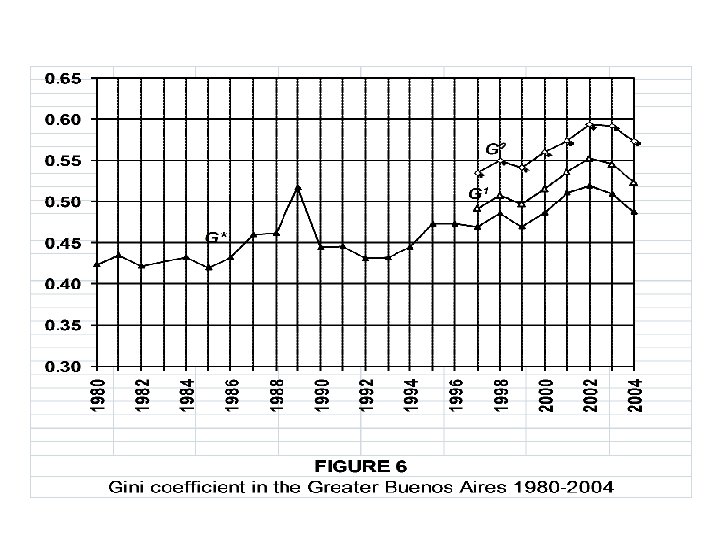
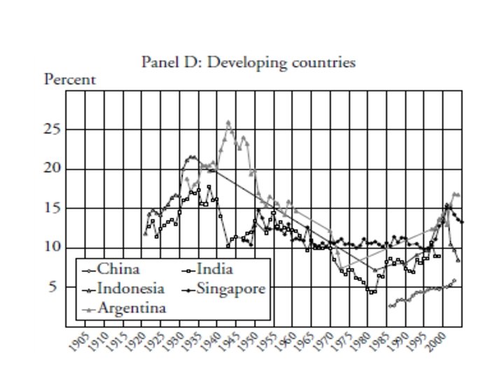
Appendix: Argentina: Share of top 1 percent over XXth century From 1930 s to 2000 s: inverted U to a U Alvaredo and Piketty, chapter 4, in Lopez- Calva and Lustig (2010)