Decision Trees n n n Decision tree representation

Decision Trees n n n Decision tree representation Top Down Construction Avoiding overfitting: Bottom up pruning Cost complexity issues (Regularization) Missing values Different construction criteria 3/22/04

Credits n n Marek A. Perkowski http: //www. ece. pdx. edu/~mperkows/ Padraig Cunningham http: //www. cs. tcd. ie/Padraig. Cunningham/aic 3/22/04 2

Supplimentary material www n n http: //dms. irb. hr/tutorial/tut_dtrees. php http: //www. cs. uregina. ca/~dbd/cs 831/notes/ ml/dtrees/4_dtrees 1. html Mitchell – Chapter 3 3/22/04 3

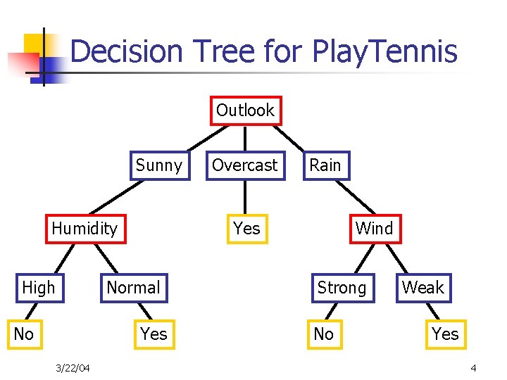
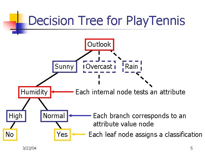
Decision Tree for Play. Tennis Outlook Sunny Humidity High No Rain Yes Normal Yes 3/22/04 Overcast Wind Strong No Weak Yes 4

Decision Tree for Play. Tennis Outlook Sunny Humidity High No Rain Each internal node tests an attribute Normal Yes 3/22/04 Overcast Each branch corresponds to an attribute value node Each leaf node assigns a classification 5

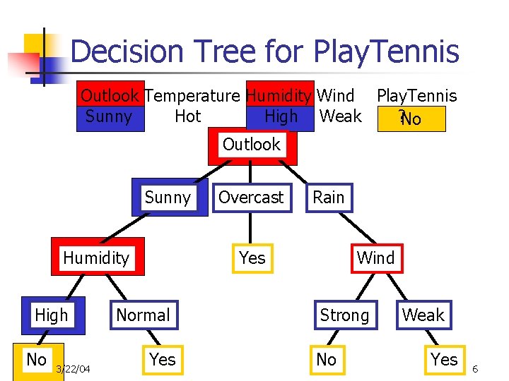
Decision Tree for Play. Tennis Outlook Temperature Humidity Wind Play. Tennis Sunny Hot High Weak ? No Outlook Sunny Humidity High No 3/22/04 Overcast Rain Yes Normal Yes Wind Strong No Weak Yes 6

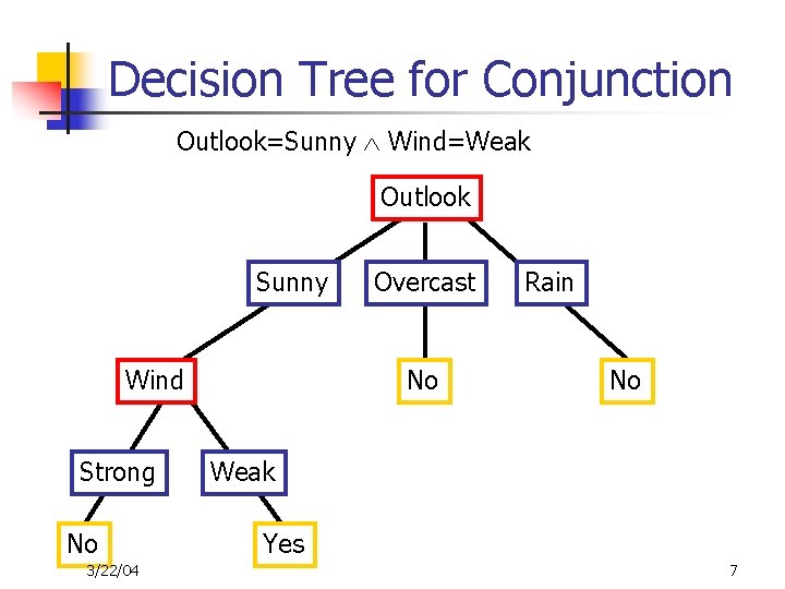
Decision Tree for Conjunction Outlook=Sunny Wind=Weak Outlook Sunny Wind Strong No 3/22/04 Overcast No Rain No Weak Yes 7

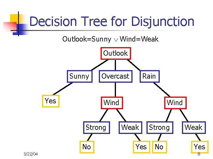
Decision Tree for Disjunction Outlook=Sunny Wind=Weak Outlook Sunny Yes Overcast Wind Strong No 3/22/04 Rain Wind Weak Yes Strong No Weak Yes 8

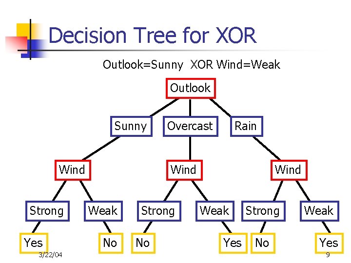
Decision Tree for XOR Outlook=Sunny XOR Wind=Weak Outlook Sunny Wind Strong Yes 3/22/04 Overcast Rain Wind Weak No Strong No Wind Weak Yes Strong No Weak Yes 9

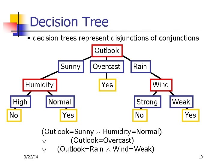
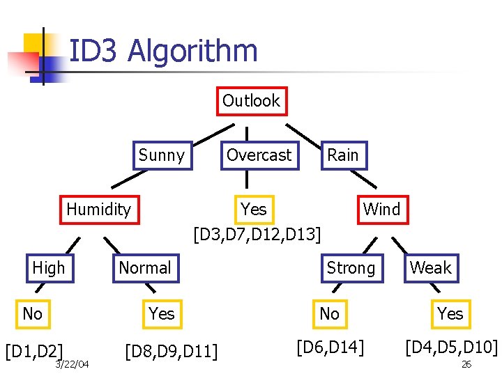
Decision Tree • decision trees represent disjunctions of conjunctions Outlook Sunny Humidity High No Overcast Rain Yes Normal Yes Wind Strong No Weak Yes (Outlook=Sunny Humidity=Normal) (Outlook=Overcast) (Outlook=Rain Wind=Weak) 3/22/04 10

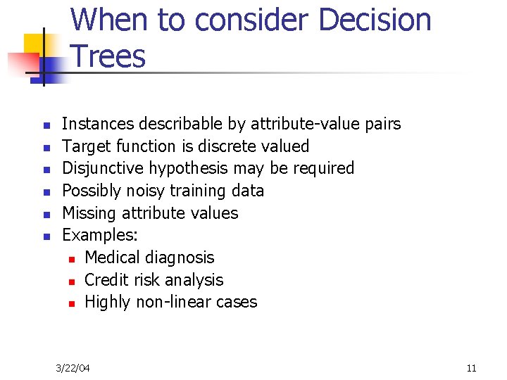
When to consider Decision Trees n n n Instances describable by attribute-value pairs Target function is discrete valued Disjunctive hypothesis may be required Possibly noisy training data Missing attribute values Examples: n Medical diagnosis n Credit risk analysis n Highly non-linear cases 3/22/04 11

History of Decision Trees n n n Quinlan developed ID 3 in early 70’s Mid 80’s Breiman et al. developed CART: Classification and Regression Trees Early 90’s Quinlan developed C 4. 5 and lately C 5. 0 (www. rulequest. com) 3/22/04 12

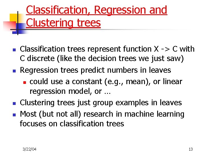
Classification, Regression and Clustering trees n n Classification trees represent function X -> C with C discrete (like the decision trees we just saw) Regression trees predict numbers in leaves n could use a constant (e. g. , mean), or linear regression model, or … Clustering trees just group examples in leaves Most (but not all) research in machine learning focuses on classification trees 3/22/04 13

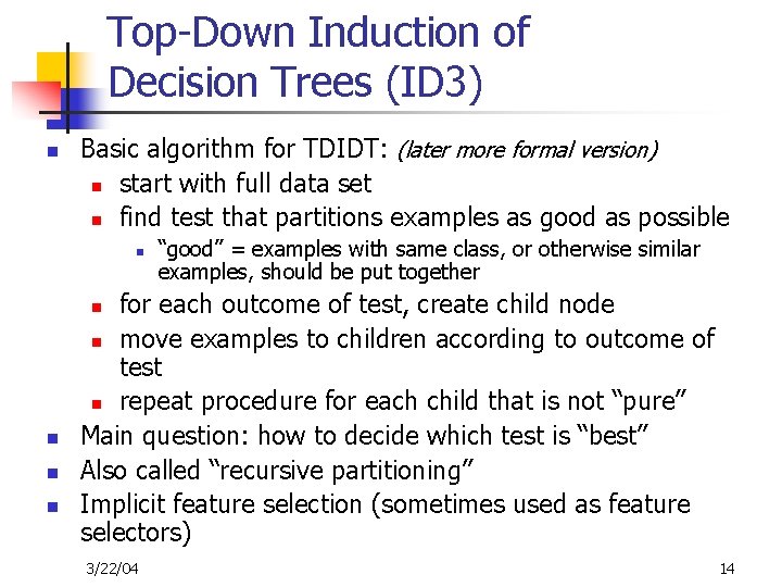
Top-Down Induction of Decision Trees (ID 3) n Basic algorithm for TDIDT: (later more formal version) n start with full data set n find test that partitions examples as good as possible n “good” = examples with same class, or otherwise similar examples, should be put together for each outcome of test, create child node n move examples to children according to outcome of test n repeat procedure for each child that is not “pure” Main question: how to decide which test is “best” Also called “recursive partitioning” Implicit feature selection (sometimes used as feature selectors) n n 3/22/04 14

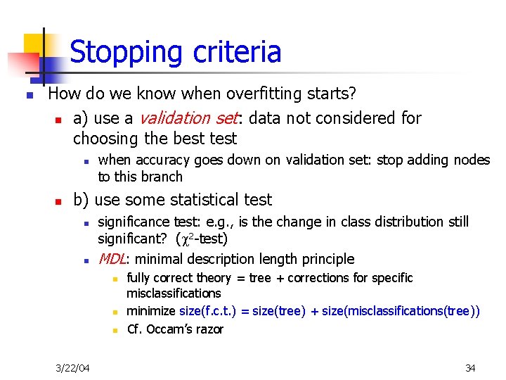
Which Attribute is ”best”? [29+, 35 -] A 1=? True [21+, 5 -] 3/22/04 A 2=? [29+, 35 -] False [8+, 30 -] True [18+, 33 -] False [11+, 2 -] 15

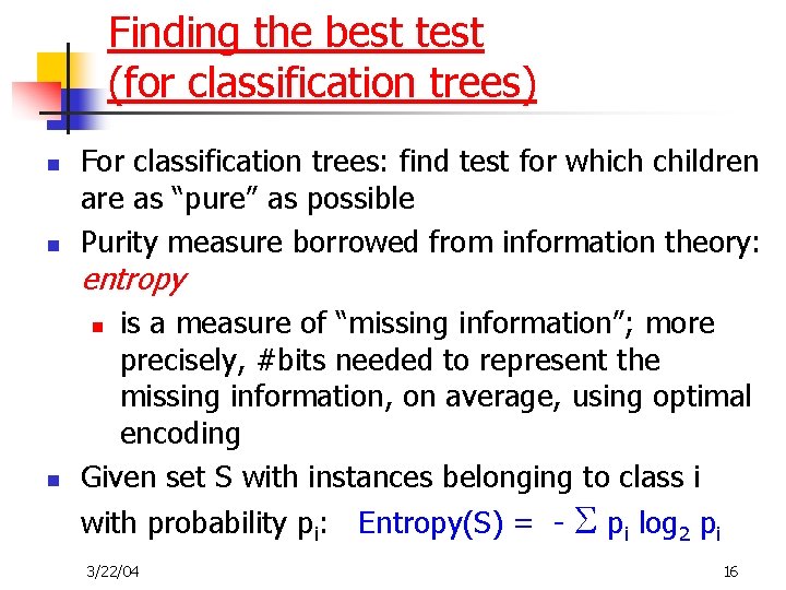
Finding the best test (for classification trees) n n For classification trees: find test for which children are as “pure” as possible Purity measure borrowed from information theory: entropy is a measure of “missing information”; more precisely, #bits needed to represent the missing information, on average, using optimal encoding Given set S with instances belonging to class i with probability pi: Entropy(S) = - pi log 2 pi n n 3/22/04 16

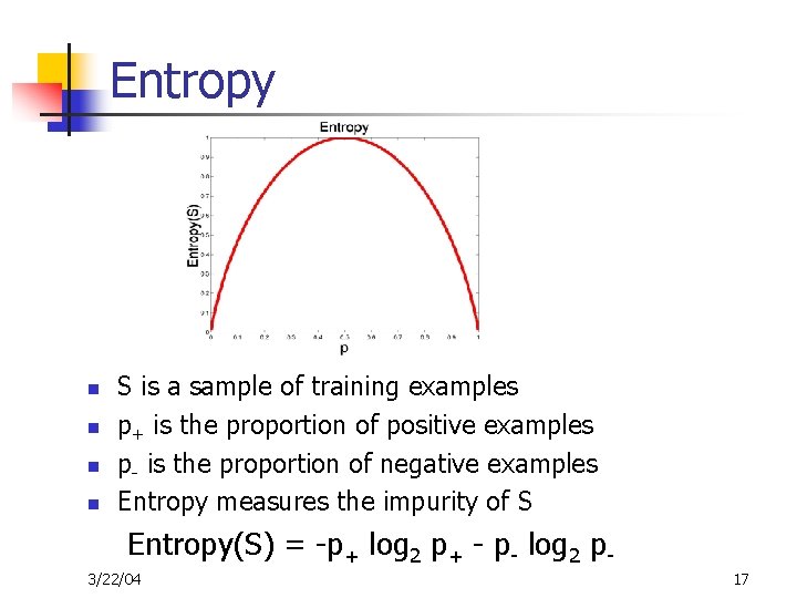
Entropy n n S is a sample of training examples p+ is the proportion of positive examples p- is the proportion of negative examples Entropy measures the impurity of S Entropy(S) = -p+ log 2 p+ - p- log 2 p 3/22/04 17

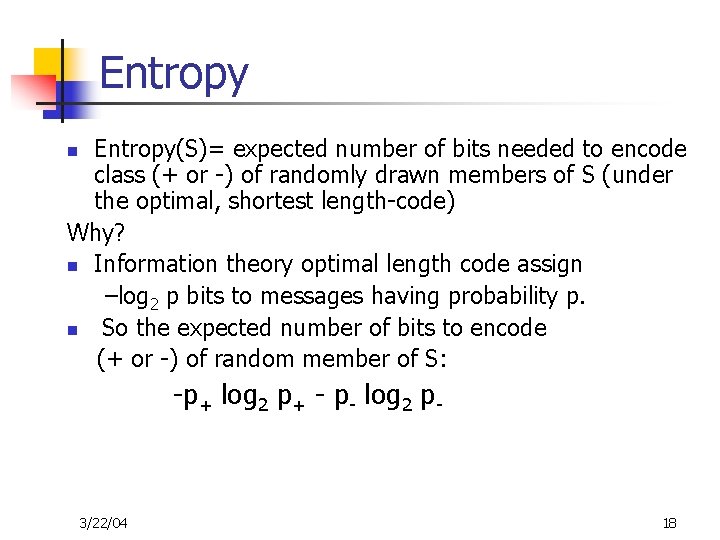
Entropy(S)= expected number of bits needed to encode class (+ or -) of randomly drawn members of S (under the optimal, shortest length-code) Why? n Information theory optimal length code assign –log 2 p bits to messages having probability p. n So the expected number of bits to encode (+ or -) of random member of S: n -p+ log 2 p+ - p- log 2 p- 3/22/04 18

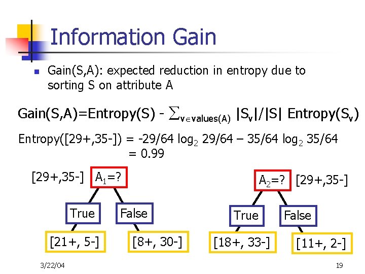
Information Gain(S, A): expected reduction in entropy due to sorting S on attribute A Gain(S, A)=Entropy(S) - v values(A) |Sv|/|S| Entropy(Sv) Entropy([29+, 35 -]) = -29/64 log 2 29/64 – 35/64 log 2 35/64 = 0. 99 [29+, 35 -] A 1=? True [21+, 5 -] 3/22/04 A 2=? [29+, 35 -] False [8+, 30 -] True [18+, 33 -] False [11+, 2 -] 19

Information Gain Entropy([21+, 5 -]) = 0. 71 Entropy([8+, 30 -]) = 0. 74 Gain(S, A 1)=Entropy(S) -26/64*Entropy([21+, 5 -]) -38/64*Entropy([8+, 30 -]) =0. 27 Entropy([18+, 33 -]) = 0. 94 Entropy([8+, 30 -]) = 0. 62 Gain(S, A 2)=Entropy(S) -51/64*Entropy([18+, 33 -]) -13/64*Entropy([11+, 2 -]) =0. 12 [29+, 35 -] A 1=? True [21+, 5 -] 3/22/04 A 2=? [29+, 35 -] False [8+, 30 -] True [18+, 33 -] False [11+, 2 -] 20

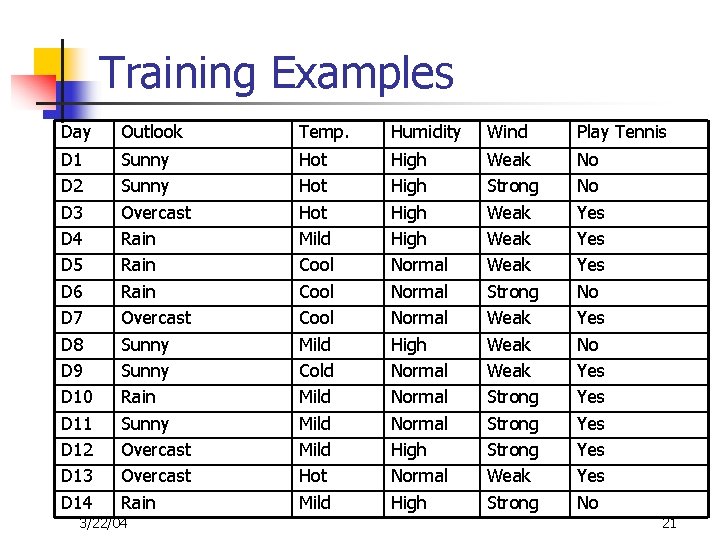
Training Examples Day Outlook Temp. Humidity Wind Play Tennis D 1 D 2 D 3 D 4 D 5 D 6 D 7 D 8 D 9 D 10 D 11 D 12 D 13 D 14 Sunny Overcast Rain Overcast Sunny Rain Sunny Overcast Rain Hot Hot Mild Cool Mild Cold Mild Hot Mild High Normal Normal High Weak Strong Weak Weak Strong Weak Strong No No Yes Yes Yes No 3/22/04 21

Selecting the Next Attribute S=[9+, 5 -] E=0. 940 Humidity Wind High [3+, 4 -] E=0. 985 Normal Weak Strong [6+, 1 -] [6+, 2 -] E=0. 592 E=0. 811 E=1. 0 Gain(S, Wind) =0. 940 -(8/14)*0. 811 – (6/14)*1. 0 =0. 048 Gain(S, Humidity) =0. 940 -(7/14)*0. 985 – (7/14)*0. 592 =0. 151 [3+, 3 -] 3/22/04 Humidity provides greater info. gain than Wind, w. r. t target classification. 22

Selecting the Next Attribute S=[9+, 5 -] E=0. 940 Outlook Sunny Over cast Rain [2+, 3 -] [4+, 0] [3+, 2 -] E=0. 971 E=0. 0 E=0. 971 Gain(S, Outlook) =0. 940 -(5/14)*0. 971 -(4/14)*0. 0 – (5/14)*0. 0971 =0. 247 3/22/04 23

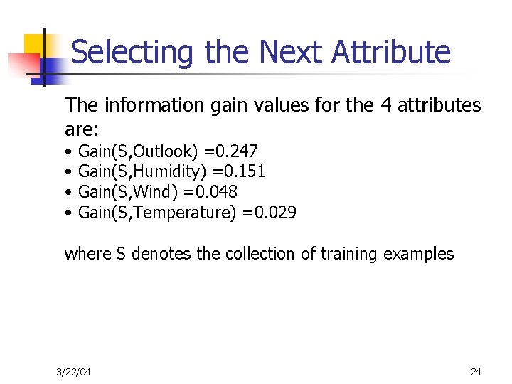
Selecting the Next Attribute The information gain values for the 4 attributes are: • • Gain(S, Outlook) =0. 247 Gain(S, Humidity) =0. 151 Gain(S, Wind) =0. 048 Gain(S, Temperature) =0. 029 where S denotes the collection of training examples 3/22/04 24

ID 3 Algorithm [D 1, D 2, …, D 14] [9+, 5 -] Outlook Sunny Overcast Rain Ssunny=[D 1, D 2, D 8, D 9, D 11] [D 3, D 7, D 12, D 13] [D 4, D 5, D 6, D 10, D 14] [2+, 3 -] [4+, 0 -] [3+, 2 -] ? Yes ? Gain(Ssunny , Humidity)=0. 970 -(3/5)0. 0 – 2/5(0. 0) = 0. 970 Gain(Ssunny , Temp. )=0. 970 -(2/5)0. 0 – 2/5(1. 0)-(1/5)0. 0 = 0. 570 Gain(Ssunny , Wind)=0. 970= -(2/5)1. 0 – 3/5(0. 918) = 0. 019 3/22/04 25

ID 3 Algorithm Outlook Sunny Humidity High No Overcast Yes [D 3, D 7, D 12, D 13] Normal Yes [D 1, D 2] 3/22/04 Rain [D 8, D 9, D 11] Wind Strong Weak No Yes [D 6, D 14] [D 4, D 5, D 10] 26

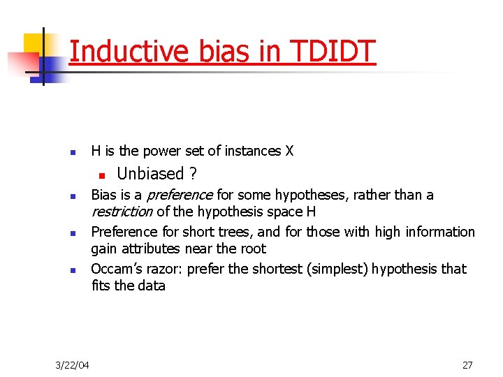
Inductive bias in TDIDT n H is the power set of instances X n n 3/22/04 Unbiased ? Bias is a preference for some hypotheses, rather than a restriction of the hypothesis space H Preference for short trees, and for those with high information gain attributes near the root Occam’s razor: prefer the shortest (simplest) hypothesis that fits the data 27

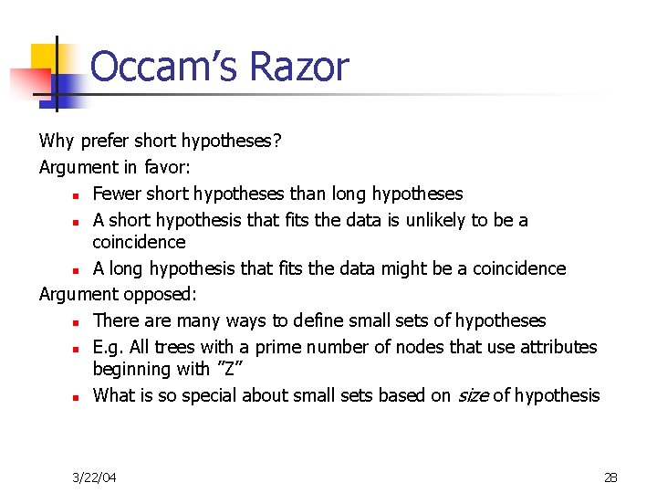
Occam’s Razor Why prefer short hypotheses? Argument in favor: n Fewer short hypotheses than long hypotheses n A short hypothesis that fits the data is unlikely to be a coincidence n A long hypothesis that fits the data might be a coincidence Argument opposed: n There are many ways to define small sets of hypotheses n E. g. All trees with a prime number of nodes that use attributes beginning with ”Z” n What is so special about small sets based on size of hypothesis 3/22/04 28

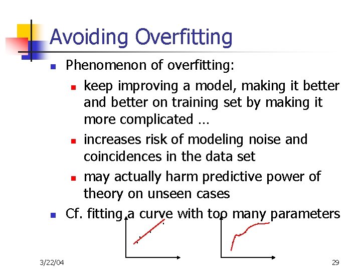
Avoiding Overfitting n n Phenomenon of overfitting: n keep improving a model, making it better and better on training set by making it more complicated … n increases risk of modeling noise and coincidences in the data set n may actually harm predictive power of theory on unseen cases Cf. fitting a curve with too many parameters. . 3/22/04 . . . . 29

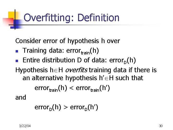
Overfitting: Definition Consider error of hypothesis h over n Training data: errortrain(h) n Entire distribution D of data: error D(h) Hypothesis h H overfits training data if there is an alternative hypothesis h’ H such that errortrain(h) < errortrain(h’) and error. D(h) > error. D(h’) 3/22/04 30

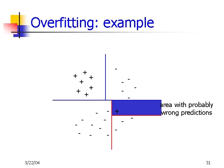
Overfitting: example - + + + + - - 3/22/04 - + - - area with probably wrong predictions - 31

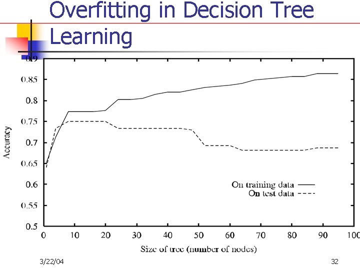
Overfitting in Decision Tree Learning 3/22/04 32

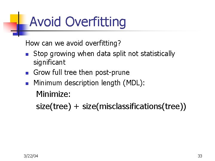
Avoid Overfitting How can we avoid overfitting? n Stop growing when data split not statistically significant n Grow full tree then post-prune n Minimum description length (MDL): Minimize: size(tree) + size(misclassifications(tree)) 3/22/04 33

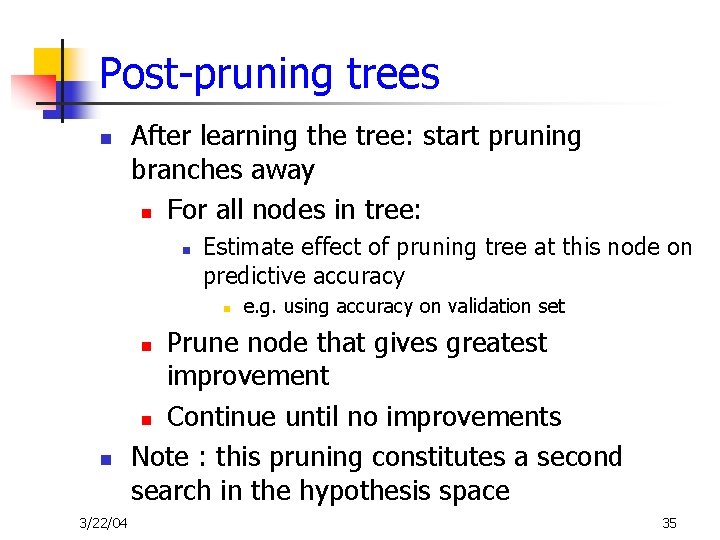
Stopping criteria n How do we know when overfitting starts? n a) use a validation set: data not considered for choosing the best test n n when accuracy goes down on validation set: stop adding nodes to this branch b) use some statistical test n n significance test: e. g. , is the change in class distribution still significant? ( 2 -test) MDL: minimal description length principle n n n 3/22/04 fully correct theory = tree + corrections for specific misclassifications minimize size(f. c. t. ) = size(tree) + size(misclassifications(tree)) Cf. Occam’s razor 34

Post-pruning trees n After learning the tree: start pruning branches away n For all nodes in tree: n Estimate effect of pruning tree at this node on predictive accuracy n e. g. using accuracy on validation set Prune node that gives greatest improvement n Continue until no improvements Note : this pruning constitutes a second search in the hypothesis space n n 3/22/04 35

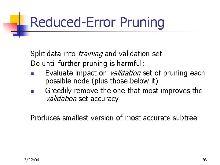
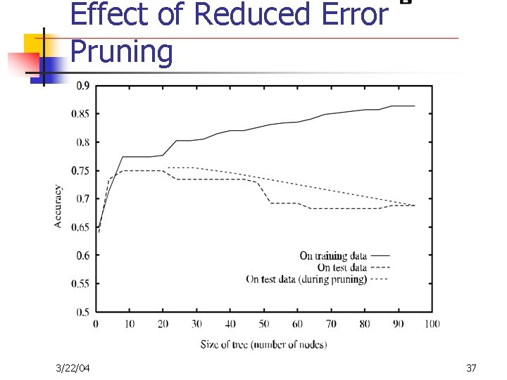
Reduced-Error Pruning Split data into training and validation set Do until further pruning is harmful: n Evaluate impact on validation set of pruning each possible node (plus those below it) n Greedily remove the one that most improves the validation set accuracy Produces smallest version of most accurate subtree 3/22/04 36

Effect of Reduced Error Pruning 3/22/04 37

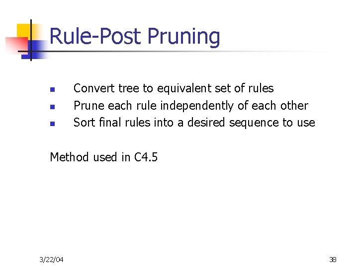
Rule-Post Pruning n n n Convert tree to equivalent set of rules Prune each rule independently of each other Sort final rules into a desired sequence to use Method used in C 4. 5 3/22/04 38

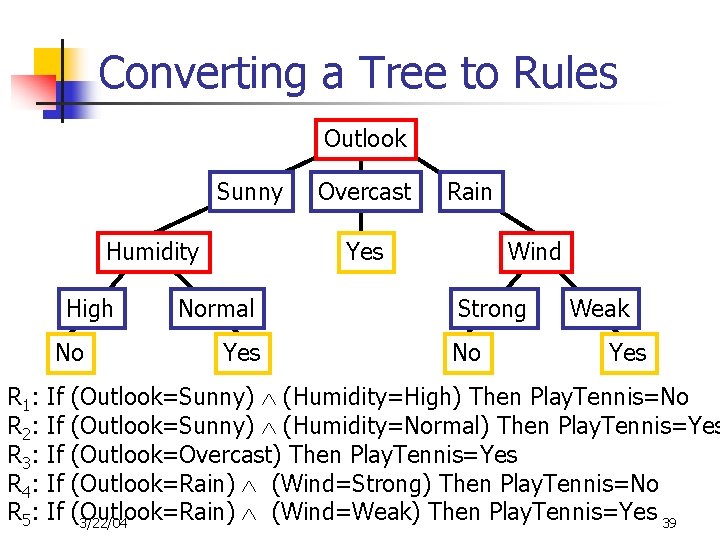
Converting a Tree to Rules Outlook Sunny Humidity High No R 1: R 2: R 3: R 4: R 5: If If If Overcast Rain Yes Normal Yes Wind Strong No Weak Yes (Outlook=Sunny) (Humidity=High) Then Play. Tennis=No (Outlook=Sunny) (Humidity=Normal) Then Play. Tennis=Yes (Outlook=Overcast) Then Play. Tennis=Yes (Outlook=Rain) (Wind=Strong) Then Play. Tennis=No (Outlook=Rain) (Wind=Weak) Then Play. Tennis=Yes 39 3/22/04

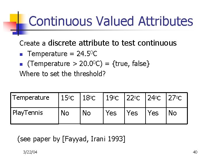
Continuous Valued Attributes Create a discrete attribute to test continuous n Temperature = 24. 50 C n (Temperature > 20. 00 C) = {true, false} Where to set the threshold? Temperature 150 C 180 C 190 C 220 C 240 C 270 C Play. Tennis No No Yes Yes No (see paper by [Fayyad, Irani 1993] 3/22/04 40

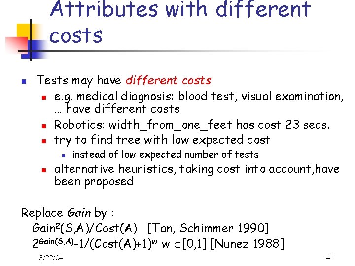
Attributes with different costs n Tests may have different costs n e. g. medical diagnosis: blood test, visual examination, … have different costs n Robotics: width_from_one_feet has cost 23 secs. n try to find tree with low expected cost n n instead of low expected number of tests alternative heuristics, taking cost into account, have been proposed Replace Gain by : Gain 2(S, A)/Cost(A) [Tan, Schimmer 1990] 2 Gain(S, A)-1/(Cost(A)+1)w w [0, 1] [Nunez 1988] 3/22/04 41

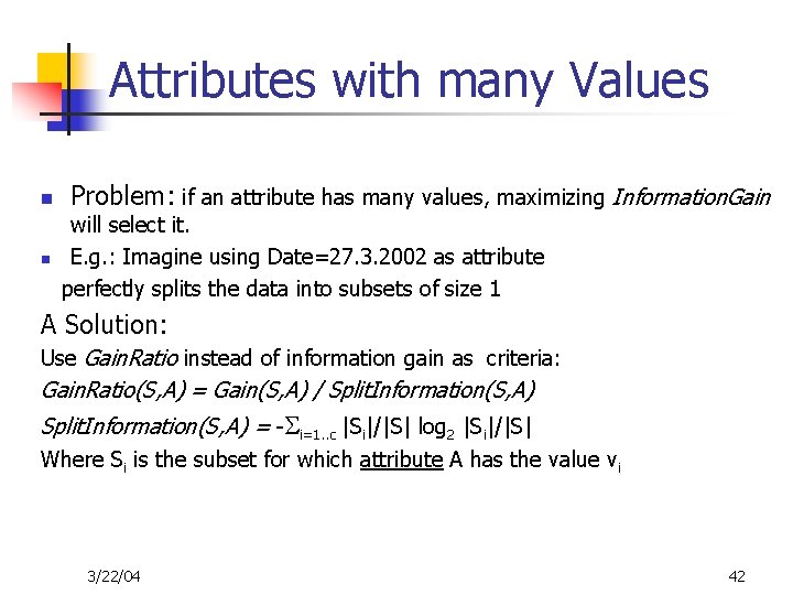
Attributes with many Values n n Problem: if an attribute has many values, maximizing Information. Gain will select it. E. g. : Imagine using Date=27. 3. 2002 as attribute perfectly splits the data into subsets of size 1 A Solution: Use Gain. Ratio instead of information gain as criteria: Gain. Ratio(S, A) = Gain(S, A) / Split. Information(S, A) = - i=1. . c |Si|/|S| log 2 |Si|/|S| Where Si is the subset for which attribute A has the value vi 3/22/04 42

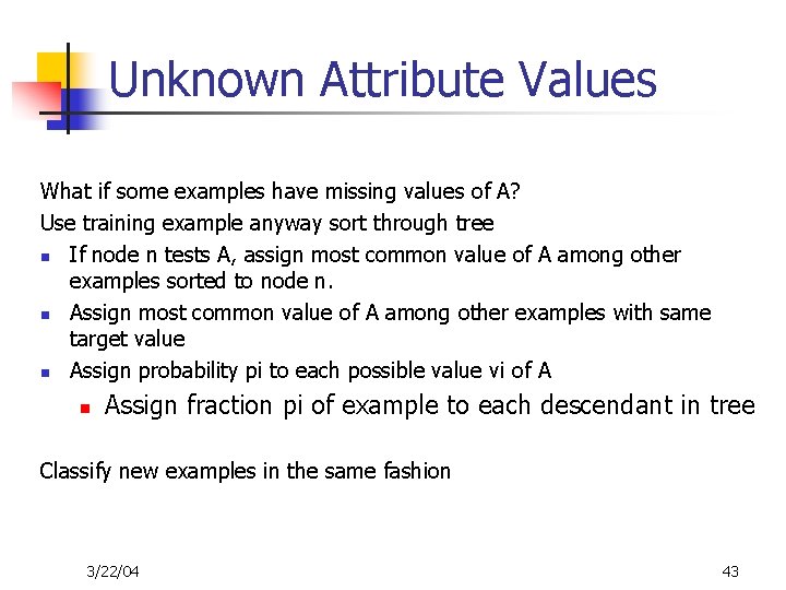
Unknown Attribute Values What if some examples have missing values of A? Use training example anyway sort through tree n If node n tests A, assign most common value of A among other examples sorted to node n. n Assign most common value of A among other examples with same target value n Assign probability pi to each possible value vi of A n Assign fraction pi of example to each descendant in tree Classify new examples in the same fashion 3/22/04 43