Decision Trees Example of a Decision Tree al

Decision Trees

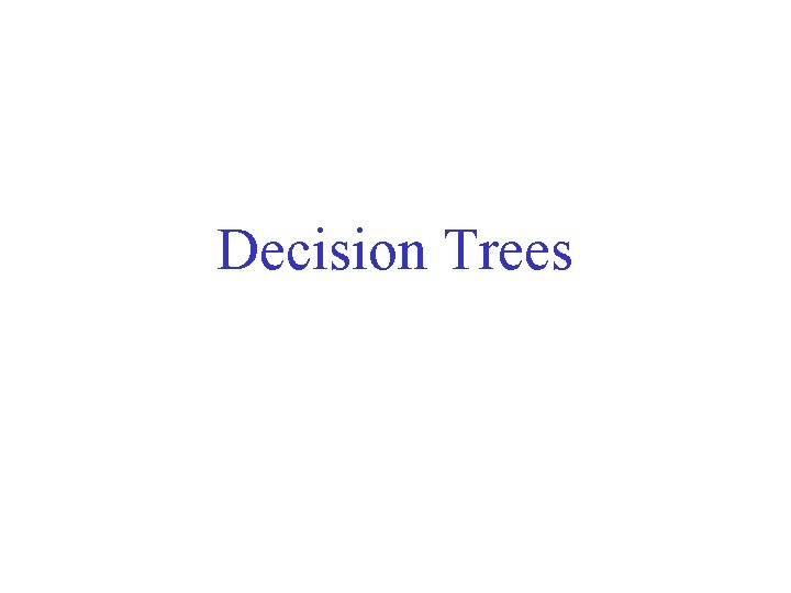
Example of a Decision Tree al ric c at o eg c at al o eg ric in nt co u s u o ss a cl Splitting Attributes Refund Yes No NO Mar. St Single, Divorced Tax. Inc < 80 K NO Training Data Married NO > 80 K YES Model: Decision Tree

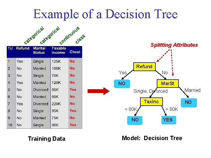
Another Example of Decision Tree l ca g te l a ric o o ca g te s a ric u uo co in t n ss a cl Married Mar. St NO Single, Divorced Refund No Yes NO Tax. Inc < 80 K NO > 80 K YES There could be more than one tree that fits the same data!

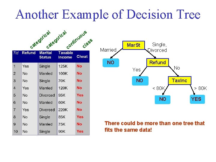
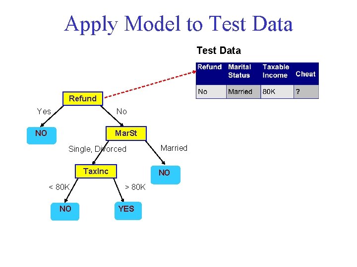
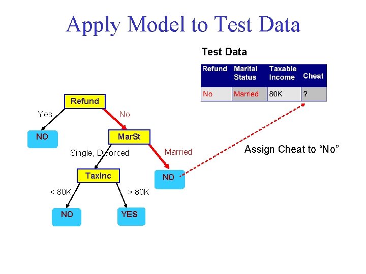
Apply Model to Test Data Start from the root of tree. Refund Yes No NO Mar. St Single, Divorced Tax. Inc < 80 K NO Married NO > 80 K YES

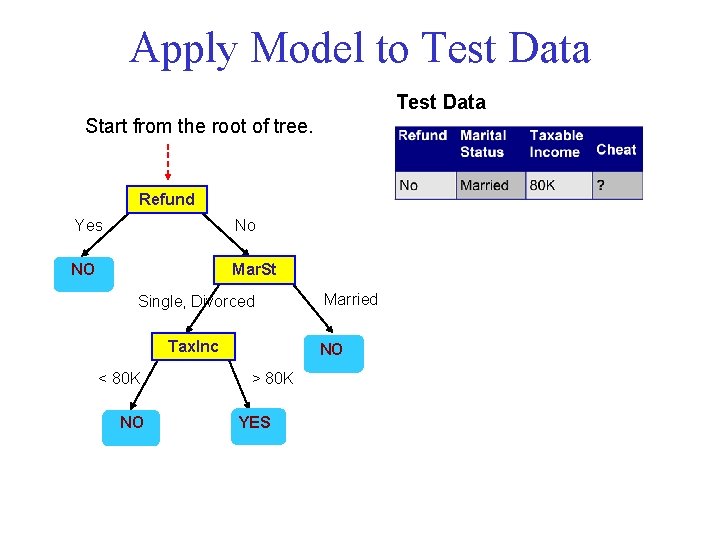
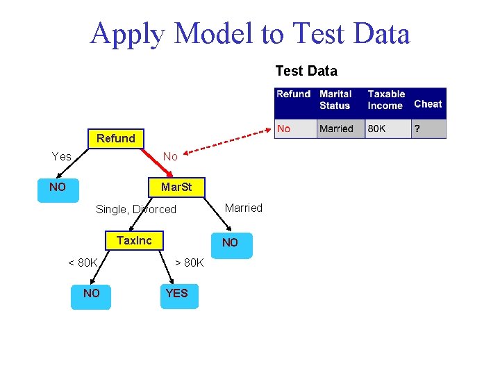
Apply Model to Test Data Refund Yes No NO Mar. St Single, Divorced Tax. Inc < 80 K NO Married NO > 80 K YES

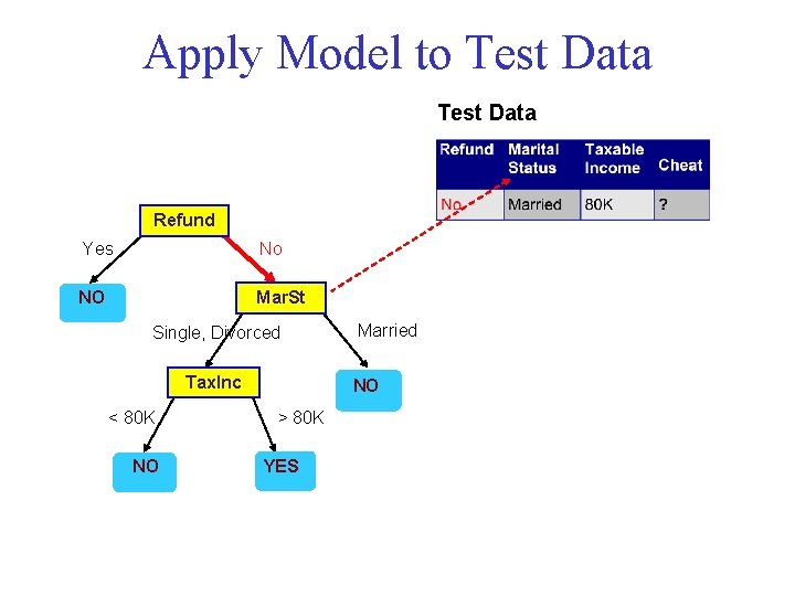
Apply Model to Test Data Refund Yes No NO Mar. St Single, Divorced Tax. Inc < 80 K NO Married NO > 80 K YES

Apply Model to Test Data Refund Yes No NO Mar. St Single, Divorced Tax. Inc < 80 K NO Married NO > 80 K YES

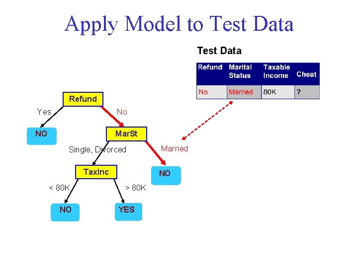
Apply Model to Test Data Refund Yes No NO Mar. St Single, Divorced Tax. Inc < 80 K NO Married NO > 80 K YES

Apply Model to Test Data Refund Yes No NO Mar. St Single, Divorced Tax. Inc < 80 K NO Married NO > 80 K YES Assign Cheat to “No”

Digression: Entropy

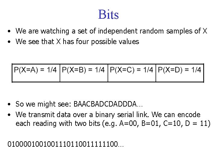
Bits • We are watching a set of independent random samples of X • We see that X has four possible values • So we might see: BAACBADCDADDDA… • We transmit data over a binary serial link. We can encode each reading with two bits (e. g. A=00, B=01, C=10, D = 11) 0100001001001110110011111100…

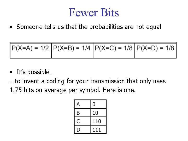
Fewer Bits • Someone tells us that the probabilities are not equal • It’s possible… …to invent a coding for your transmission that only uses 1. 75 bits on average per symbol. Here is one.

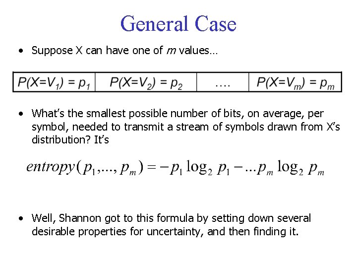
General Case • Suppose X can have one of m values… • What’s the smallest possible number of bits, on average, per symbol, needed to transmit a stream of symbols drawn from X’s distribution? It’s • Well, Shannon got to this formula by setting down several desirable properties for uncertainty, and then finding it.

Back to Decision Trees

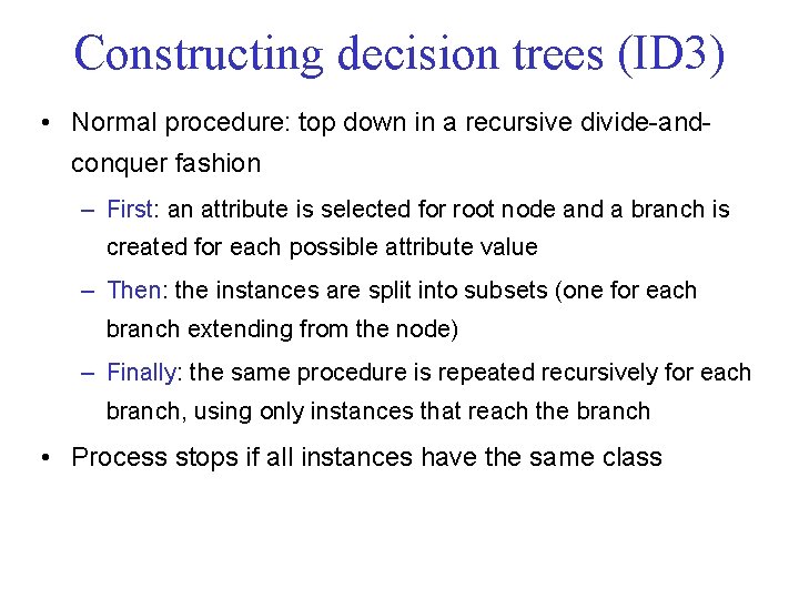
Constructing decision trees (ID 3) • Normal procedure: top down in a recursive divide-andconquer fashion – First: an attribute is selected for root node and a branch is created for each possible attribute value – Then: the instances are split into subsets (one for each branch extending from the node) – Finally: the same procedure is repeated recursively for each branch, using only instances that reach the branch • Process stops if all instances have the same class

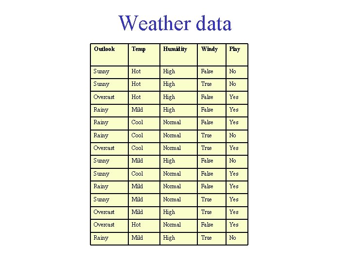
Weather data Outlook Temp Humidity Windy Play Sunny Hot High False No Sunny Hot High True No Overcast Hot High False Yes Rainy Mild High False Yes Rainy Cool Normal True No Overcast Cool Normal True Yes Sunny Mild High False No Sunny Cool Normal False Yes Rainy Mild Normal False Yes Sunny Mild Normal True Yes Overcast Mild High True Yes Overcast Hot Normal False Yes Rainy Mild High True No

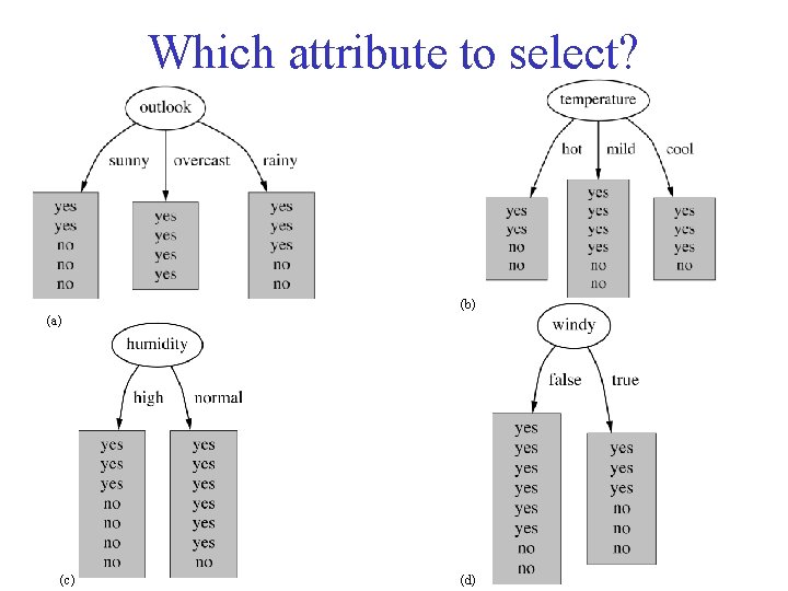
Which attribute to select? (b) (a) (c) (d)

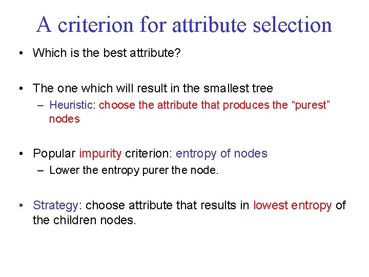
A criterion for attribute selection • Which is the best attribute? • The one which will result in the smallest tree – Heuristic: choose the attribute that produces the “purest” nodes • Popular impurity criterion: entropy of nodes – Lower the entropy purer the node. • Strategy: choose attribute that results in lowest entropy of the children nodes.

Attribute “Outlook” outlook=sunny info([2, 3]) = entropy(2/5, 3/5) = -2/5*log(2/5) -3/5*log(3/5) =. 971 outlook=overcast info([4, 0]) = entropy(4/4, 0/4) = -1*log(1) -0*log(0) = 0 0*log(0) is normally not defined. outlook=rainy info([3, 2]) = entropy(3/5, 2/5) = -3/5*log(3/5)-2/5*log(2/5) =. 971 Expected info: . 971*(5/14) + 0*(4/14) +. 971*(5/14) =. 693

Attribute “Temperature” temperature=hot info([2, 2]) = entropy(2/4, 2/4) = -2/4*log(2/4) = 1 temperature=mild info([4, 2]) = entropy(4/6, 2/6) = -4/6*log(1) -2/6*log(2/6) =. 528 temperature=cool info([3, 1]) = entropy(3/4, 1/4) = -3/4*log(3/4)-1/4*log(1/4) =. 811 Expected info: 1*(4/14) +. 528*(6/14) +. 811*(4/14) =. 744

Attribute “Humidity” humidity=high info([3, 4]) = entropy(3/7, 4/7) = -3/7*log(3/7) -4/7*log(4/7) =. 985 humidity=normal info([6, 1]) = entropy(6/7, 1/7) = -6/7*log(6/7) -1/7*log(1/7) =. 592 Expected info: . 985*(7/14) +. 592*(7/14) =. 788

Attribute “Windy” windy=false info([6, 2]) = entropy(6/8, 2/8) = -6/8*log(6/8) -2/8*log(2/8) =. 811 humidity=true info([3, 3]) = entropy(3/6, 3/6) = -3/6*log(3/6) = 1 Expected info: . 811*(8/14) + 1*(6/14) =. 892

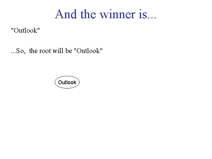
And the winner is. . . "Outlook". . . So, the root will be "Outlook" Outlook

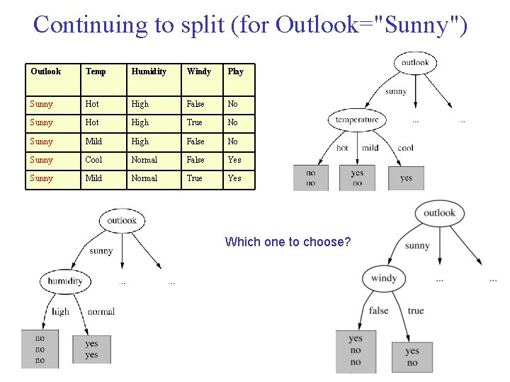
Continuing to split (for Outlook="Sunny") Outlook Temp Humidity Windy Play Sunny Hot High False No Sunny Hot High True No Sunny Mild High False No Sunny Cool Normal False Yes Sunny Mild Normal True Yes Which one to choose?

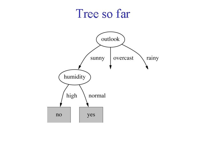
Continuing to split (for Outlook="Sunny") temperature=hot: info([2, 0]) = entropy(2/2, 0/2) = 0 temperature=mild: info([1, 1]) = entropy(1/2, 1/2) = 1 temperature=cool: info([1, 0]) = entropy(1/1, 0/1) = 0 Expected info: 0*(2/5) + 1*(2/5) + 0*(1/5) =. 4 humidity=high: info([3, 0]) = 0 humidity=normal: info([2, 0]) = 0 Expected info: 0 windy=false: info([1, 2]) = entropy(1/3, 2/3) = -1/3*log(1/3) -2/3*log(2/3) =. 918 humidity=true: info([1, 1]) = entropy(1/2, 1/2) = 1 Expected info: . 918*(3/5) + 1*(2/5) =. 951 Winner is "humidity"

Tree so far

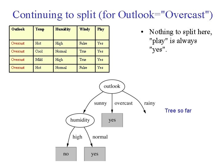
Continuing to split (for Outlook="Overcast") Outlook Temp Humidity Windy Play Overcast Hot High False Yes Overcast Cool Normal True Yes Overcast Mild High True Yes Overcast Hot Normal False Yes • Nothing to split here, "play" is always "yes". Tree so far

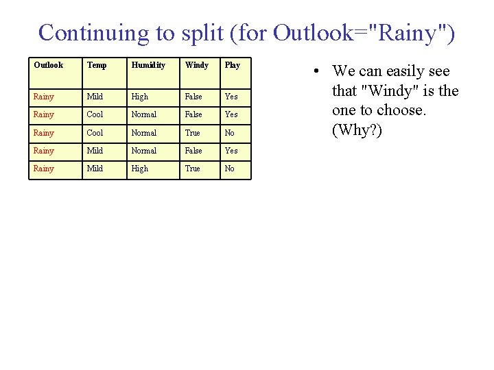
Continuing to split (for Outlook="Rainy") Outlook Temp Humidity Windy Play Rainy Mild High False Yes Rainy Cool Normal True No Rainy Mild Normal False Yes Rainy Mild High True No • We can easily see that "Windy" is the one to choose. (Why? )

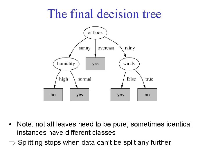
The final decision tree • Note: not all leaves need to be pure; sometimes identical instances have different classes Þ Splitting stops when data can’t be split any further

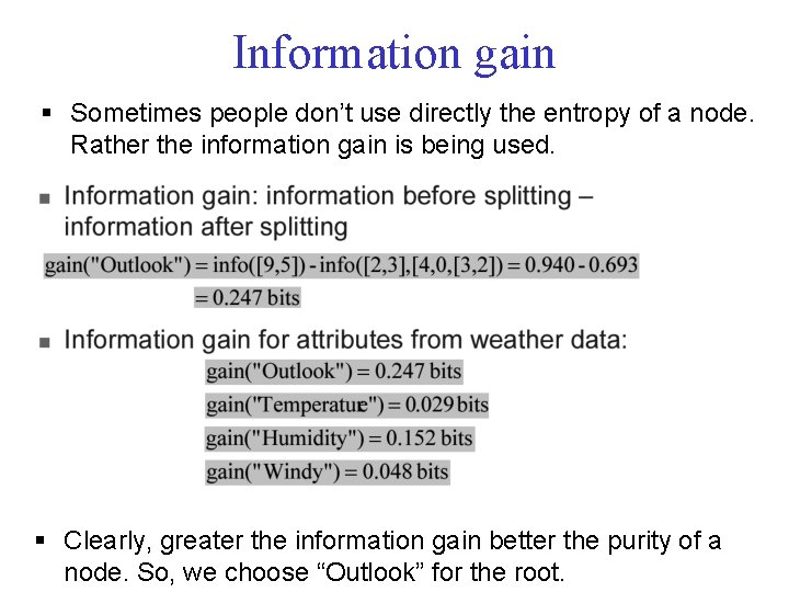
Information gain § Sometimes people don’t use directly the entropy of a node. Rather the information gain is being used. § Clearly, greater the information gain better the purity of a node. So, we choose “Outlook” for the root.

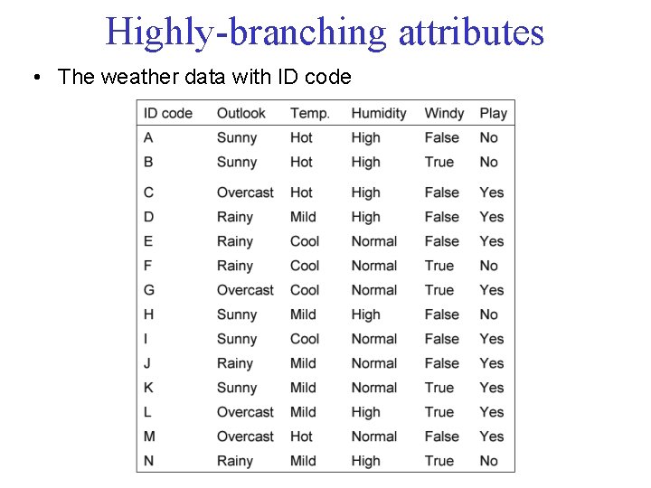
Highly-branching attributes • The weather data with ID code

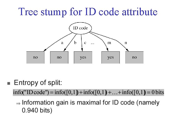
Tree stump for ID code attribute

Highly-branching attributes So, • Subsets are more likely to be pure if there is a large number of values – Information gain is biased towards choosing attributes with a large number of values – This may result in overfitting (selection of an attribute that is non-optimal for prediction)

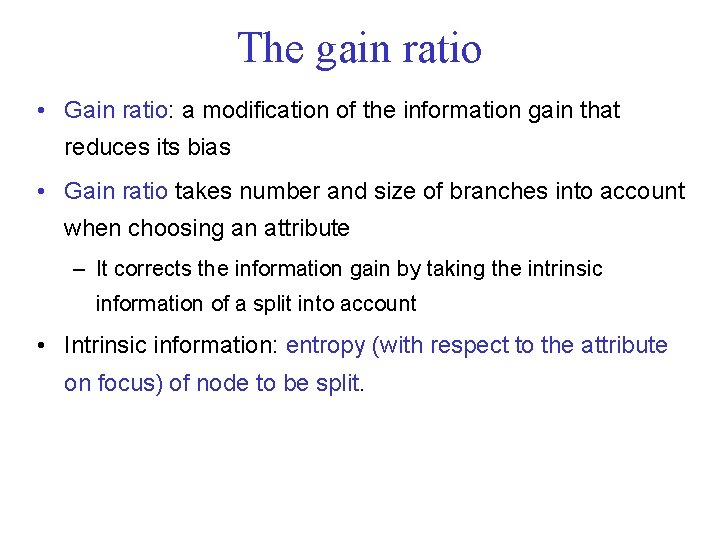
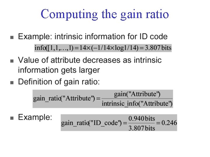
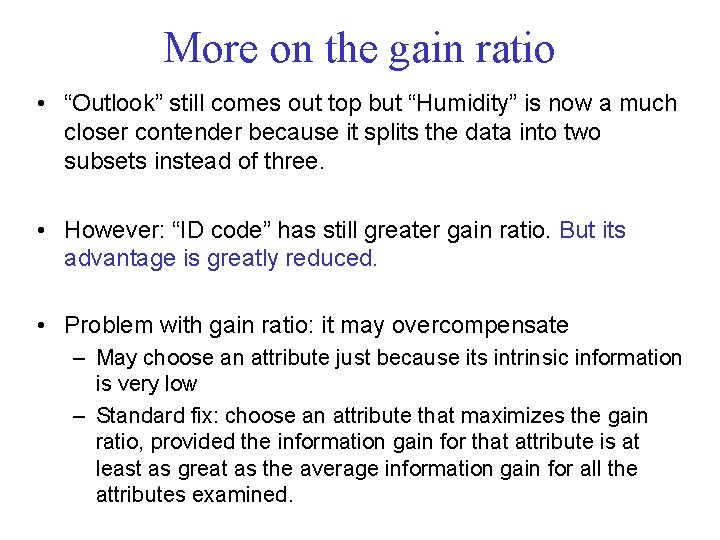
The gain ratio • Gain ratio: a modification of the information gain that reduces its bias • Gain ratio takes number and size of branches into account when choosing an attribute – It corrects the information gain by taking the intrinsic information of a split into account • Intrinsic information: entropy (with respect to the attribute on focus) of node to be split.

Computing the gain ratio

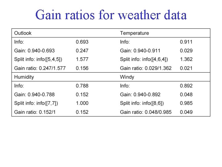
Gain ratios for weather data

More on the gain ratio • “Outlook” still comes out top but “Humidity” is now a much closer contender because it splits the data into two subsets instead of three. • However: “ID code” has still greater gain ratio. But its advantage is greatly reduced. • Problem with gain ratio: it may overcompensate – May choose an attribute just because its intrinsic information is very low – Standard fix: choose an attribute that maximizes the gain ratio, provided the information gain for that attribute is at least as great as the average information gain for all the attributes examined.

Discussion • Algorithm for top-down induction of decision trees (“ID 3”) was developed by Ross Quinlan (University of Sydney Australia) • Gain ratio is just one modification of this basic algorithm – Led to development of C 4. 5, which can deal with numeric attributes, missing values, and noisy data • There are many other attribute selection criteria! (But almost no difference in accuracy of result. )