Decision Trees and Decision Tree Learning Philipp Krger

Decision Trees and Decision Tree Learning Philipp Kärger

Outline: 1. Decision Trees 2. Decision Tree Learning 1. ID 3 Algorithm 2. Which attribute to split on? 3. Some examples 3. Overfitting 4. Where to use Decision Trees?

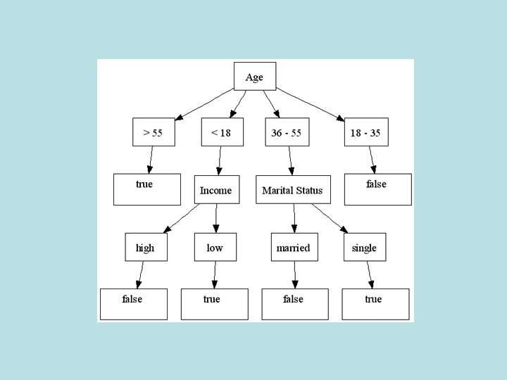
Decision tree representation for Play. Tennis Outlook Sunny Overcast Humidity High No Rain Yes Normal Yes Wind Strong No Weak Yes

Decision tree representation for Play. Tennis Outlook Attribute Sunny Overcast Humidity High No Rain Yes Normal Yes Wind Strong No Weak Yes

Decision tree representation for Play. Tennis Outlook Value Sunny Overcast Humidity High No Rain Yes Normal Yes Wind Strong No Weak Yes

Decision tree representation for Play. Tennis Outlook Classification Sunny Overcast Humidity High No Rain Yes Normal Yes Wind Strong No Weak Yes

Play. Tennis: Other representations • Logical expression for Play. Tennis=Yes: – (Outlook=Sunny Humidity=Normal) (Outlook=Overcast) (Outlook=Rain Wind=Weak) • If-then rules – IF Outlook=Sunny Humidity=Normal THEN Play. Tennis=Yes – IF Outlook=Overcast THEN Play. Tennis=Yes – IF Outlook=Rain Wind=Weak THEN Play. Tennis=Yes – IF Outlook=Sunny Humidity=High THEN Play. Tennis=No – IF Outlook=Rain Wind=Strong THEN Play. Tennis=Yes

Decision Trees - Summary • a model of a part of the world • allows us to classify instances (by performing a sequence of tests) • allows us to predict classes of (unseen) instances • understandable by humans (unlike many other representations)

Decision Tree Learning

• Goal: Learn from known instances how to classify unseen instances • by means of building and exploiting a Decision Tree • supervised or unsupervised learning?

Application: classification of medical patients by their disease Classification Task seen patients Decision Tree unseen patients check attributes of an unseen patient rules telling which attributes of the patient indicates a disease

Basic algorithm: ID 3 (simplified) ID 3 = Iterative Dichotomiser 3 - given a goal class to build the tree for A 1=weather A 2=day happy sun odd yes rain odd no rain even no - create a root node for the tree sun even - if all examples from the test set belong to the same goal class C rain odd then label the root with C sun even - else – select the ‘most informative’ attribute A – split the training set according to the values V 1. . Vn of A – recursively build the resulting subtrees T 1 … Tn – generate decision tree T: A v 1 . . . vn yes no yes Humidity Low High T 1 . . . Tn No Yes

• lessons learned: – there is always more than one decision tree – finding the “best” one is NP complete – all the known algorithms use heuristics • finding the right attribute A to split on is tricky

Search heuristics in ID 3 • Which attribute should we split on? • Need a heuristic – Some function gives big numbers for “good” splits • Want to get to “pure” sets • How can we measure “pure”? odd even sunny rain

Measuring Information: Entropy • The average amount of information I needed to classify an object is given by the entropy measure p(c) = probability of class Cc (sum over all classes) • For a two-class problem: entropy p(c)

• What is the entropy of the set of happy/unhappy days? A 1=weather A 2=day happy sun odd yes odd rain odd no even rain even no sun even yes rain odd no sun even yes sunny rain

Residual Information • After applying attribute A, S is partitioned into subsets according to values v of A • Ires represents the amount of information still needed to classify an instance • Ires is equal to weighted sum of the amounts of information for the subsets p(c|v) = probability that an instance belongs to class C given that it belongs to v = I(v)

• What is Ires(A) if I split for “weather” and if I split for “day”? A 1=weather A 2=day happy sun odd yes rain odd no rain even no sun even yes rain odd no sun even yes Ires(weather) = 0 Ires(day) = 1 odd even sunny rain

Information Gain: = the amount of information I rule out by splitting on attribute A: Gain(A) = I – Ires(A) = information in the current set minus the residual information after splitting The most ‘informative’ attribute is the one that minimizes Ires, i. e. , maximizes the Gain

Triangles and Squares Data Set: A set of classified objects. . .

Entropy. . . • 5 triangles • 9 squares • class probabilities. • entropy of the data set

Entropy reduction by data set partitioning . . . . red Color? green . yellow . . .

residual information . . . . red Color? green yellow . .

Information Gain . . . . red Color? green yellow . .

Information Gain of The Attribute • Attributes – Gain(Color) = 0. 246 – Gain(Outline) = 0. 151 – Gain(Dot) = 0. 048 • Heuristics: attribute with the highest gain is chosen • This heuristics is local (local minimization of impurity)

. . . . red Color? green . . yellow . . Gain(Outline) = 0. 971 – 0 = 0. 971 bits Gain(Dot) = 0. 971 – 0. 951 = 0. 020 bits

. . . . red Gain(Outline) = 0. 971 – 0. 951 = 0. 020 bits Gain(Dot) = 0. 971 – 0 = 0. 971 bits Color? green . . yellow . . solid Outline? dashed . .

. . . . red . yes Dot? Color? . no green . . yellow . . solid Outline? dashed . .

Decision Tree. . . Color red Dot yes triangle yellow green square no square Outline dashed triangle solid square

A Defect of Ires • Ires favors attributes with many values • Such attribute splits S to many subsets, and if these are small, they will tend to be pure anyway • One way to rectify this is through a corrected measure of information gain ratio. A 1=weather A 2=day happy sun 17. 1. 08 yes rain 18. 1. 08 no rain 19. 1. 08 no sun 20. 1. 08 yes sun 21. 1. 08 yes

Information Gain Ratio • I(A) is amount of information needed to determine the value of an attribute A • Information gain ratio

Information Gain Ratio . . . . red Color? green yellow . .

Information Gain and Information Gain Ratio

Overfitting (Example)

Overfitting Underfitting: when model is too simple, both training and test errors are large

Notes on Overfitting • Overfitting results in decision trees that are more complex than necessary • Training error no longer provides a good estimate of how well the tree will perform on previously unseen records

How to Address Overfitting Idea: prune the tree so that it is not too specific Two possibilities: Pre-Pruning - prune while building the tree Post-Pruning - prune after building the tree

How to Address Overfitting • Pre-Pruning (Early Stopping Rule) – Stop the algorithm before it becomes a fullygrown tree – More restrictive stopping conditions: • Stop if number of instances is less than some userspecified threshold • Stop if expanding the current node does not improve impurity measures (e. g. , information gain). – Not successful in practice

How to Address Overfitting… • Post-pruning – Grow decision tree to its entirety – Trim the nodes of the decision tree in a bottom-up fashion – If generalization error improves after trimming, replace sub-tree by a leaf node. – Class label of leaf node is determined from majority class of instances in the sub-tree

Occam’s Razor • Given two models of similar generalization errors, one should prefer the simpler model over the more complex model • For complex models, there is a greater chance that it was fitted accidentally by errors in data • Therefore, one should prefer less complex models in general

When to use Decision Tree Learning?

Appropriate problems for decision tree learning • Classification problems • Characteristics: – – instances described by attribute-value pairs target function has discrete output values training data may be noisy training data may contain missing attribute values

Strengths • • can generate understandable rules perform classification without much computation can handle continuous and categorical variables provide a clear indication of which fields are most important for prediction or classification

Weakness • Not suitable for prediction of continuous attribute. • Perform poorly with many class and small data. • Computationally expensive to train. – At each node, each candidate splitting field must be sorted before its best split can be found. – In some algorithms, combinations of fields are used and a search must be made for optimal combining weights. – Pruning algorithms can also be expensive since many potential sub-trees must be formed and compared