Decision Trees AMT NOTICE Proprietary and Confidential This

Decision Trees AMT NOTICE: Proprietary and Confidential This material is proprietary to A. Teredesai and GCCIS, RIT. Slide 1 amt@cs. rit. edu Proprietary and Confidential

Overview Decision trees Appropriate problems for decision trees Entropy and Information Gain The ID 3 algorithm Avoiding Overfitting via Pruning Handling Continuous Valued Attributes Handling Missing Attribute Values Alternative Measures for Selecting Attributes amt@cs. rit. edu Dr. Ankur M. Teredesai P 2

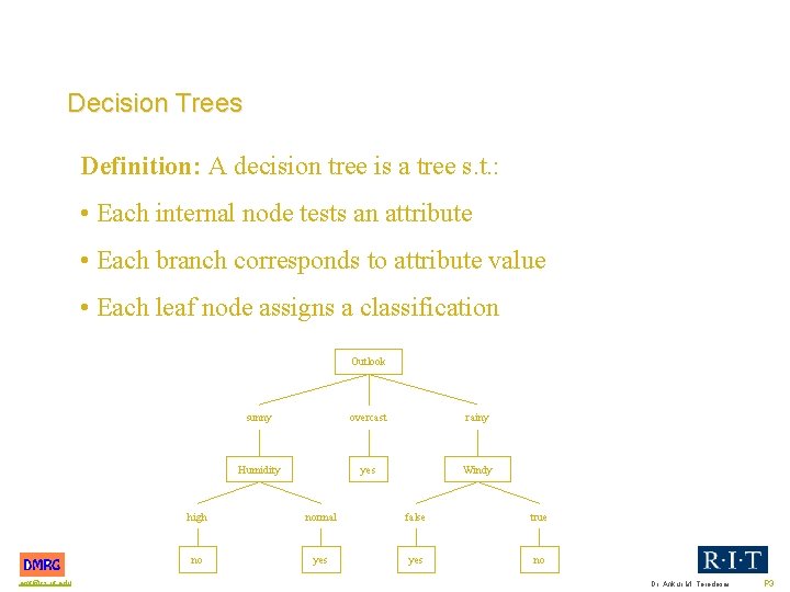
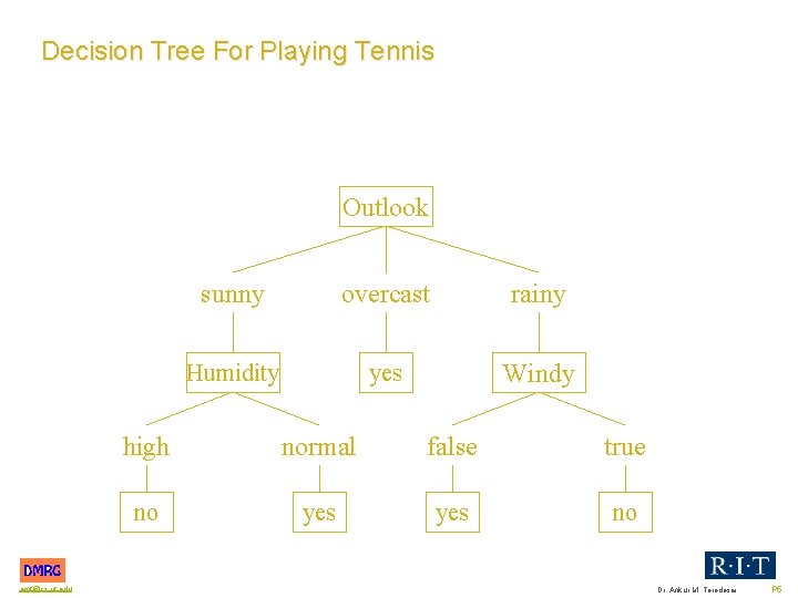
Decision Trees Definition: A decision tree is a tree s. t. : • Each internal node tests an attribute • Each branch corresponds to attribute value • Each leaf node assigns a classification Outlook amt@cs. rit. edu sunny overcast rainy Humidity yes Windy high normal false true no yes no Dr. Ankur M. Teredesai P 3

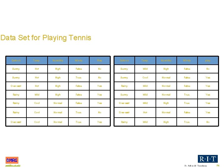
Data Set for Playing Tennis Outlook Temp. Humidity Windy Play Outlook Temp. Humidity Windy play Sunny Hot High False No Sunny Mild High False No Sunny Hot High True No Sunny Cool Normal False Yes Overcast Hot High False Yes Rainy Mild Normal False Yes Rainy Mild High False Yes Sunny Mild Normal True Yes Rainy Cool Normal False Yes Overcast Mild High True Yes Rainy Cool Normal True No Overcast Hot Normal False Yes Overcast Cool Normal True Yes Rainy Mild High True No amt@cs. rit. edu Dr. Ankur M. Teredesai P 4

Decision Tree For Playing Tennis Outlook amt@cs. rit. edu sunny overcast rainy Humidity yes Windy high normal false true no yes no Dr. Ankur M. Teredesai P 5

When to Consider Decision Trees Each instance consists of an attribute with discrete values (e. g. outlook/sunny, etc. . ) The classification is over discrete values (e. g. yes/no ) It is okay to have disjunctive descriptions – each path in the tree represents a disjunction of attribute combinations. Any Boolean function can be represented! It is okay for the training data to contain errors – decision trees are robust to classification errors in the training data. It is okay for the training data to contain missing values – decision trees can be used even if instances have missing attributes. amt@cs. rit. edu Dr. Ankur M. Teredesai P 6

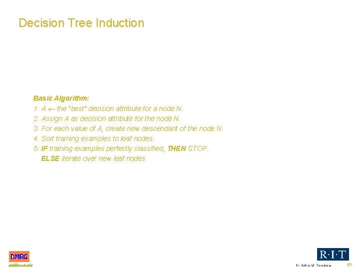
Decision Tree Induction Basic Algorithm: 1. A the “best" decision attribute for a node N. 2. Assign A as decision attribute for the node N. 3. For each value of A, create new descendant of the node N. 4. Sort training examples to leaf nodes. 5. IF training examples perfectly classified, THEN STOP. ELSE iterate over new leaf nodes amt@cs. rit. edu Dr. Ankur M. Teredesai P 7

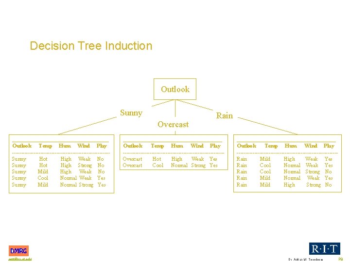
Decision Tree Induction Outlook Sunny Overcast __________________ Outlook Temp Hum Wind Play ---------------------------Sunny Hot High Weak No Sunny Hot High Strong No Sunny Mild High Weak No Sunny Cool Normal Weak Yes Sunny Mild Normal Strong Yes amt@cs. rit. edu Rain ___________________ Outlook Temp Hum Wind Play ----------------------------Overcast Hot High Weak Yes Overcast Cool Normal Strong Yes ___________________ Outlook Temp Hum Wind Play ----------------------------Rain Mild High Weak Yes Rain Cool Normal Strong No Rain Mild Normal Weak Yes Rain Mild High Strong No Dr. Ankur M. Teredesai P 8

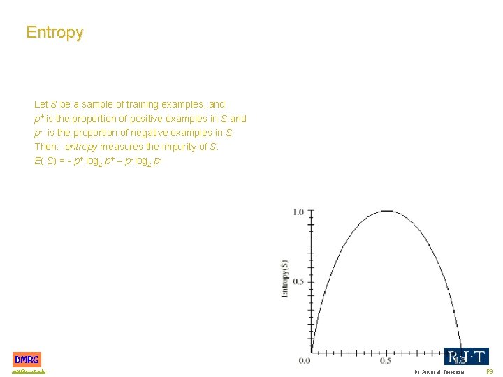
Entropy Let S be a sample of training examples, and p+ is the proportion of positive examples in S and p- is the proportion of negative examples in S. Then: entropy measures the impurity of S: E( S) = p+ log 2 p+ – p- log 2 p- amt@cs. rit. edu Dr. Ankur M. Teredesai P 9

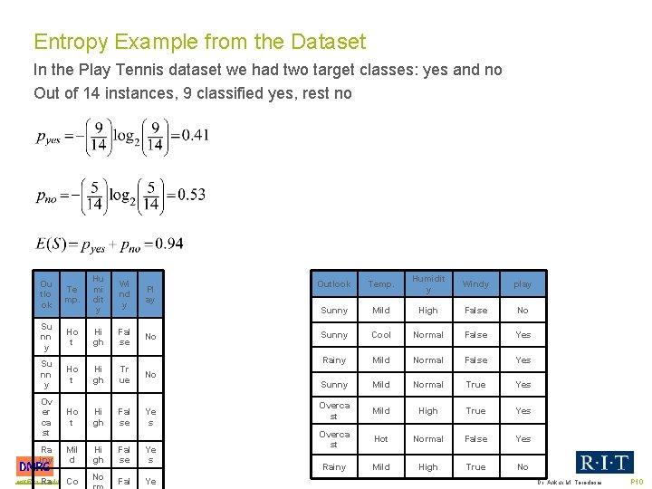
Entropy Example from the Dataset In the Play Tennis dataset we had two target classes: yes and no Out of 14 instances, 9 classified yes, rest no Hu mi dit y Wi nd y Pl ay Ho t Hi gh Fal se No Su nn y Ho t Hi gh Tr ue No Ov er ca st Ho t Hi gh Fal se Ye s Ra iny Mil d Ou tlo ok Te mp. Su nn y amt@cs. rit. edu Ra Co Hi gh No Fal se Ye s Fal Ye Outlook Temp. Humidit y Windy play Sunny Mild High False No Sunny Cool Normal False Yes Rainy Mild Normal False Yes Sunny Mild Normal True Yes Overca st Mild High True Yes Overca st Hot Normal False Yes Rainy Mild High True No Dr. Ankur M. Teredesai P 10

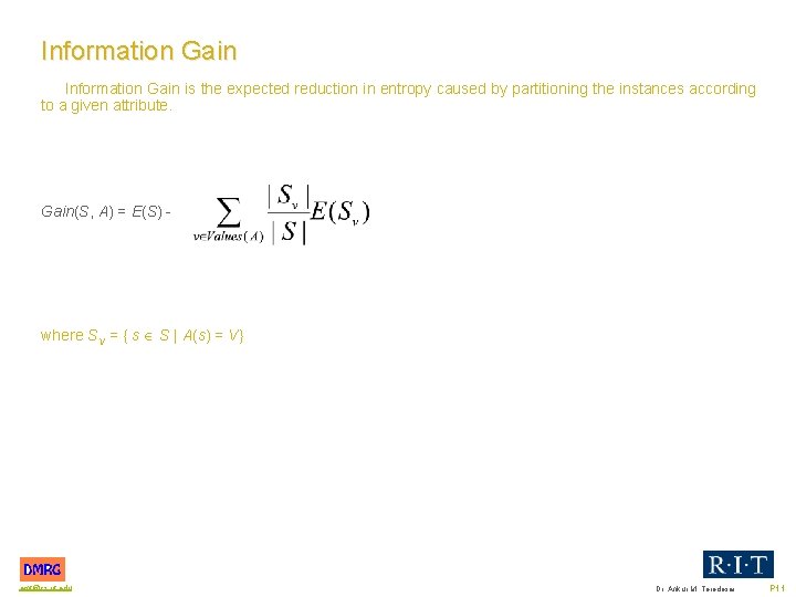
Information Gain is the expected reduction in entropy caused by partitioning the instances according to a given attribute. Gain(S, A) = E(S) where SV = { s S | A(s) = V} amt@cs. rit. edu Dr. Ankur M. Teredesai P 11

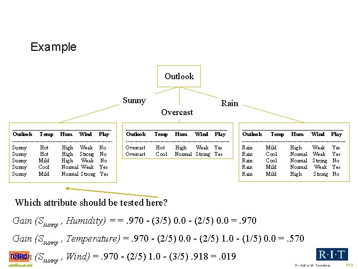
Example Outlook Sunny Overcast __________________ Outlook Temp Hum Wind Play ---------------------------Sunny Hot High Weak No Sunny Hot High Strong No Sunny Mild High Weak No Sunny Cool Normal Weak Yes Sunny Mild Normal Strong Yes Rain ___________________ Outlook Temp Hum Wind Play ----------------------------Overcast Hot High Weak Yes Overcast Cool Normal Strong Yes ___________________ Outlook Temp Hum Wind Play ----------------------------Rain Mild High Weak Yes Rain Cool Normal Strong No Rain Mild Normal Weak Yes Rain Mild High Strong No Which attribute should be tested here? Gain (Ssunny , Humidity) = =. 970 - (3/5) 0. 0 - (2/5) 0. 0 =. 970 Gain (Ssunny , Temperature) =. 970 - (2/5) 0. 0 - (2/5) 1. 0 - (1/5) 0. 0 =. 570 Gain (Ssunny , Wind) =. 970 - (2/5) 1. 0 - (3/5). 918 =. 019 amt@cs. rit. edu Dr. Ankur M. Teredesai P 12

ID 3 Algorithm Informally: • Determine the attribute with the highest information gain on the training set. • Use this attribute as the root, create a branch for each of the values the attribute can have. • For each branch, repeat the process with subset of the training set that is classified by that branch. amt@cs. rit. edu Dr. Ankur M. Teredesai P 13

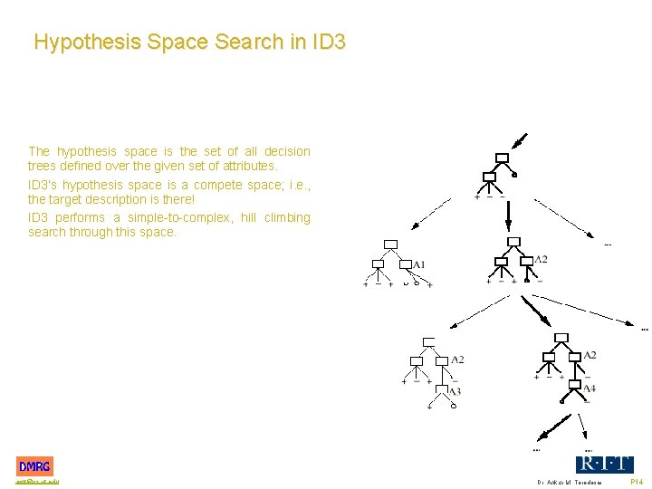
Hypothesis Space Search in ID 3 The hypothesis space is the set of all decision trees defined over the given set of attributes. ID 3’s hypothesis space is a compete space; i. e. , the target description is there! ID 3 performs a simple to complex, hill climbing search through this space. amt@cs. rit. edu Dr. Ankur M. Teredesai P 14

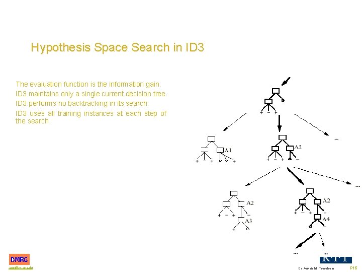
Hypothesis Space Search in ID 3 The evaluation function is the information gain. ID 3 maintains only a single current decision tree. ID 3 performs no backtracking in its search. ID 3 uses all training instances at each step of the search. amt@cs. rit. edu Dr. Ankur M. Teredesai P 15

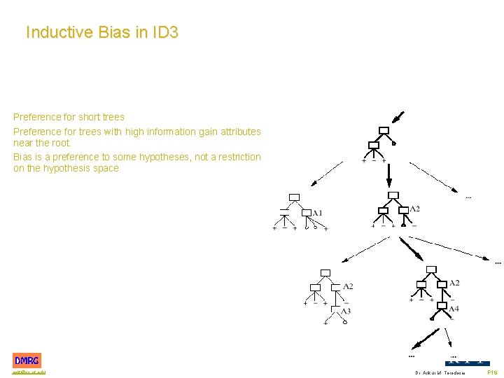
Inductive Bias in ID 3 Preference for short trees Preference for trees with high information gain attributes near the root. Bias is a preference to some hypotheses, not a restriction on the hypothesis space amt@cs. rit. edu Dr. Ankur M. Teredesai P 16

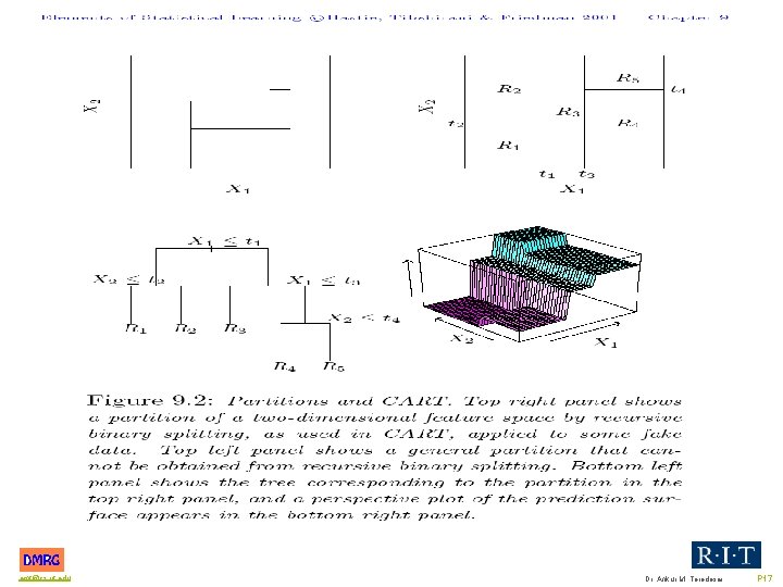
amt@cs. rit. edu Dr. Ankur M. Teredesai P 17

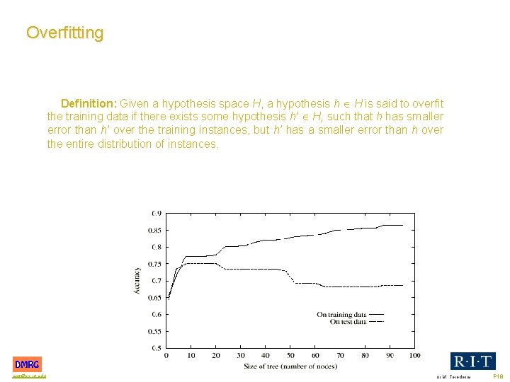
Overfitting Definition: Given a hypothesis space H, a hypothesis h H is said to overfit the training data if there exists some hypothesis h’ H, such that h has smaller error than h’ over the training instances, but h’ has a smaller error than h over the entire distribution of instances. amt@cs. rit. edu Dr. Ankur M. Teredesai P 18

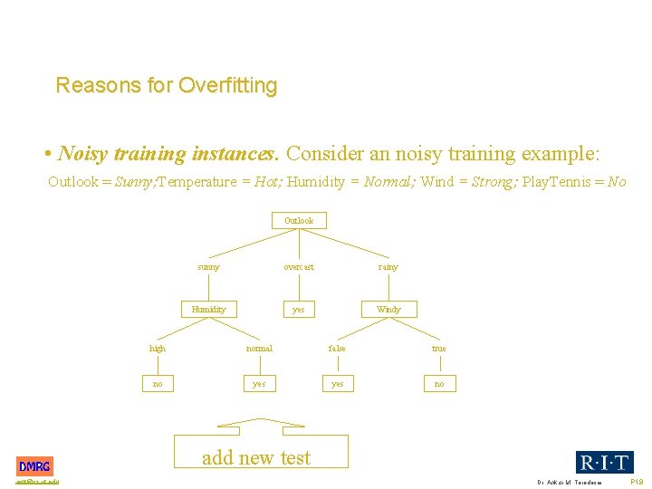
Reasons for Overfitting • Noisy training instances. Consider an noisy training example: Outlook = Sunny; Temperature = Hot; Humidity = Normal; Wind = Strong; Play. Tennis = No Outlook sunny overcast rainy Humidity yes Windy high normal false true no yes no add new test amt@cs. rit. edu Dr. Ankur M. Teredesai P 19

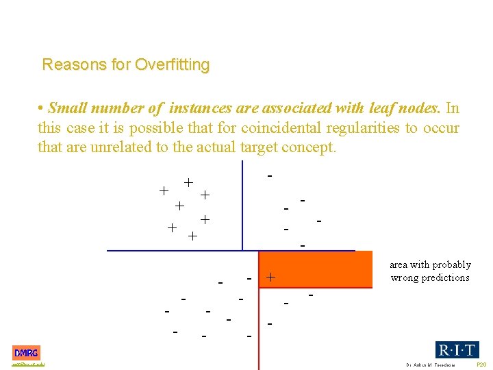
Reasons for Overfitting • Small number of instances are associated with leaf nodes. In this case it is possible that for coincidental regularities to occur that are unrelated to the actual target concept. - + + ++ - amt@cs. rit. edu - - area with probably wrong predictions - + - - - Dr. Ankur M. Teredesai P 20

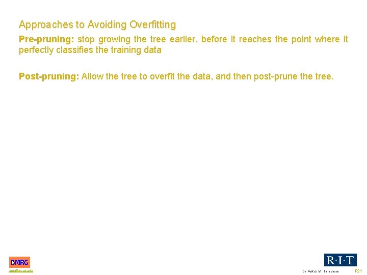
Approaches to Avoiding Overfitting Pre-pruning: stop growing the tree earlier, before it reaches the point where it perfectly classifies the training data Post-pruning: Allow the tree to overfit the data, and then post prune the tree. amt@cs. rit. edu Dr. Ankur M. Teredesai P 21

Criteria for Pruning Use a separate set of instances, distinct from the training instances, to evaluate the utility of nodes in the tree. This requires the data to be split into a training set and a validation set which is then used for pruning. The reason is that the validation set is unlikely to suffer from same errors or fluctuations as the training set. Use all the available data for training, but apply a statistical test to estimate whether expanding/pruning a particular node is likely to produce improvement beyond the training set. amt@cs. rit. edu Dr. Ankur M. Teredesai P 22

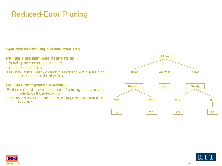
Reduced Error Pruning Split data into training and validation sets. Outlook Pruning a decision node d consists of: removing the subtree rooted at d. making d a leaf node. assigning d the most common classification of the training instances associated with d. Do until further pruning is harmful: Evaluate impact on validation set of pruning each possible node (plus those below it). Greedily remove the one that most improves validation set accuracy. amt@cs. rit. edu sunny overcast rainy Humidity yes Windy high normal false true no yes no Dr. Ankur M. Teredesai P 23

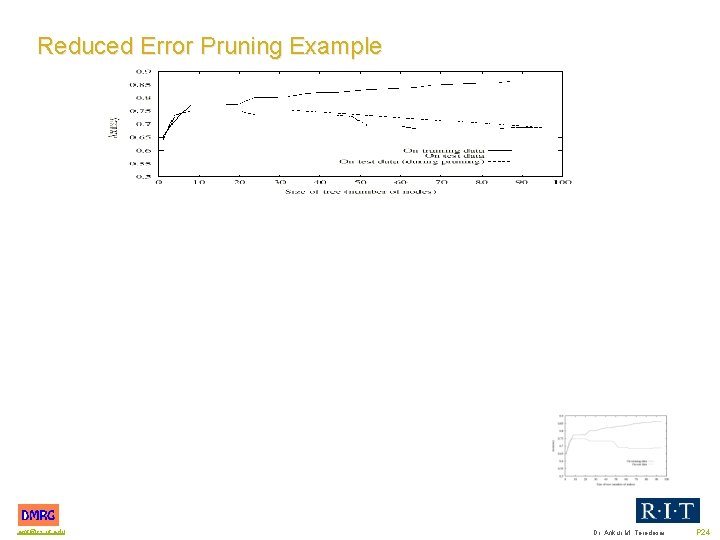
Reduced Error Pruning Example amt@cs. rit. edu Dr. Ankur M. Teredesai P 24

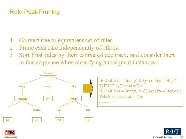
Rule Post Pruning 1. Convert tree to equivalent set of rules. 2. Prune each rule independently of others. 3. Sort final rules by their estimated accuracy, and consider them in this sequence when classifying subsequent instances. Outlook no amt@cs. rit. edu sunny overcast rainy Humidity yes Windy IF (Outlook = Sunny) & (Humidity = High) THEN Play. Tennis = No IF (Outlook = Sunny) & (Humidity = Normal) THEN Play. Tennis = Yes ………. normal false true yes no Dr. Ankur M. Teredesai P 25

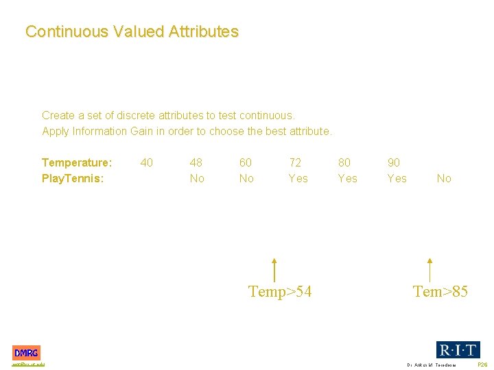
Continuous Valued Attributes Create a set of discrete attributes to test continuous. Apply Information Gain in order to choose the best attribute. Temperature: Play. Tennis: 40 48 No 60 No 72 Yes Temp>54 amt@cs. rit. edu 80 Yes 90 Yes No Tem>85 Dr. Ankur M. Teredesai P 26

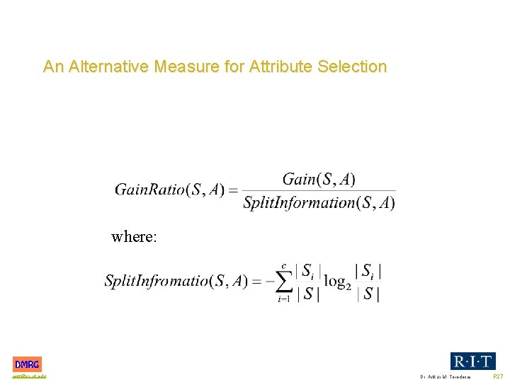
An Alternative Measure for Attribute Selection where: amt@cs. rit. edu Dr. Ankur M. Teredesai P 27

Missing Attribute Values Strategies: 1. Assign most common value of A among other examples belonging to the same concept. 2. If node n tests the attribute A, assign most common value of A among other examples sorted to node n. 3. If node n tests the attribute A, assign a probability to each of possible values of A. These probabilities are estimated based on the observed frequencies of the values of A. These probabilities are used in the information gain measure. amt@cs. rit. edu Dr. Ankur M. Teredesai P 28

Summary Points 1. Decision tree learning provides a practical method for concept learning. 2. ID 3 -like algorithms search complete hypothesis space. 3. The inductive bias of decision trees is preference (search) bias. 4. Overfitting the training data is an important issue in decision tree learning. 5. A large number of extensions of the ID 3 algorithm have been proposed for overfitting avoidance, handling missing attributes, handling numerical attributes, etc. amt@cs. rit. edu Dr. Ankur M. Teredesai P 29

References Mitchell, Tom. M. 1997. Machine Learning. New York: Mc. Graw Hill Quinlan, J. R. 1986. Induction of decision trees. Machine Learning Stuart Russell, Peter Norvig, 1995. Artificial Intelligence: A Modern Approach. New Jersey: Prantice Hall amt@cs. rit. edu Dr. Ankur M. Teredesai P 30

Rain. Forest - A Framework for Fast Decision Tree Construction of Large Datasets J. Gehrke, R. Ramakrishnan, V. Ganti Dept. of Computer Sciences University of Wisconsin-Madison NOTICE: Proprietary and Confidential This material is proprietary to A. Teredesai and GCCIS, RIT. Slide 31 amt@cs. rit. edu Proprietary and Confidential

Introduction to Classification An important Data Mining Problem Input: a database of training records – Class label attributes – Predictor Attributes Goal • to build a concise model of the distribution of class label in terms of predictor attributes Applications • scientific experiments, medical diagnosis, fraud detection, etc. amt@cs. rit. edu Dr. Ankur M. Teredesai P 32

Decision Tree: A Classification Model It is one of the most attractive classification models There a large number of algorithms to construct decision trees • E. g. : SLIQ, CART, C 4. 5 SPRINT • Most are main memory algorithms • Tradeoff between supporting large databases, performance and constructing more accurate decision trees amt@cs. rit. edu Dr. Ankur M. Teredesai P 33

Motivation of Rain. Forest Developing a unifying framework that can be applied to most decision tree algorithms, and results in a scalable version of this algorithm without modifying the results. Separating the scalability aspects of these algorithms from the central features that determine the quality of the decision trees amt@cs. rit. edu Dr. Ankur M. Teredesai P 34

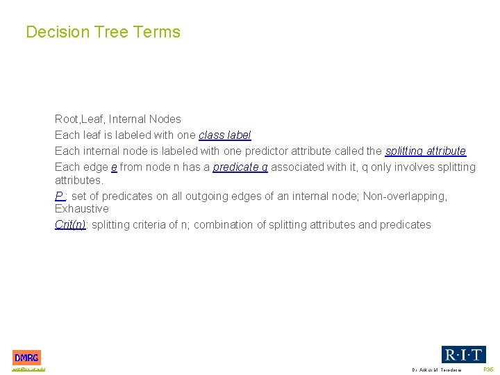
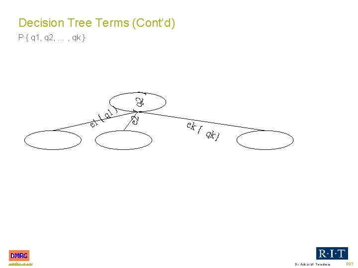
Decision Tree Terms Root, Leaf, Internal Nodes Each leaf is labeled with one class label Each internal node is labeled with one predictor attribute called the splitting attribute Each edge e from node n has a predicate q associated with it, q only involves splitting attributes. P : set of predicates on all outgoing edges of an internal node; Non overlapping, Exhaustive Crit(n): splitting criteria of n; combination of splitting attributes and predicates amt@cs. rit. edu Dr. Ankur M. Teredesai P 35

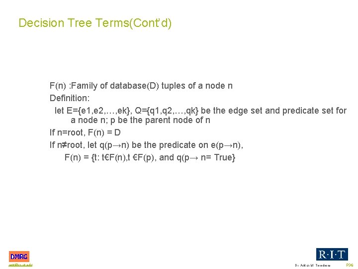
Decision Tree Terms(Cont’d) F(n) : Family of database(D) tuples of a node n Definition: let E={e 1, e 2, …, ek}, Q={q 1, q 2, …, qk} be the edge set and predicate set for a node n; p be the parent node of n If n=root, F(n) = D If n≠root, let q(p→n) be the predicate on e(p→n), F(n) = {t: t€F(n), t €F(p), and q(p→ n= True} amt@cs. rit. edu Dr. Ankur M. Teredesai P 36

Decision Tree Terms (Cont’d) 2} P { q 1, q 2, … , qk } e 1 amt@cs. rit. edu 1 {q } e 2 { q n ek { qk} Dr. Ankur M. Teredesai P 37

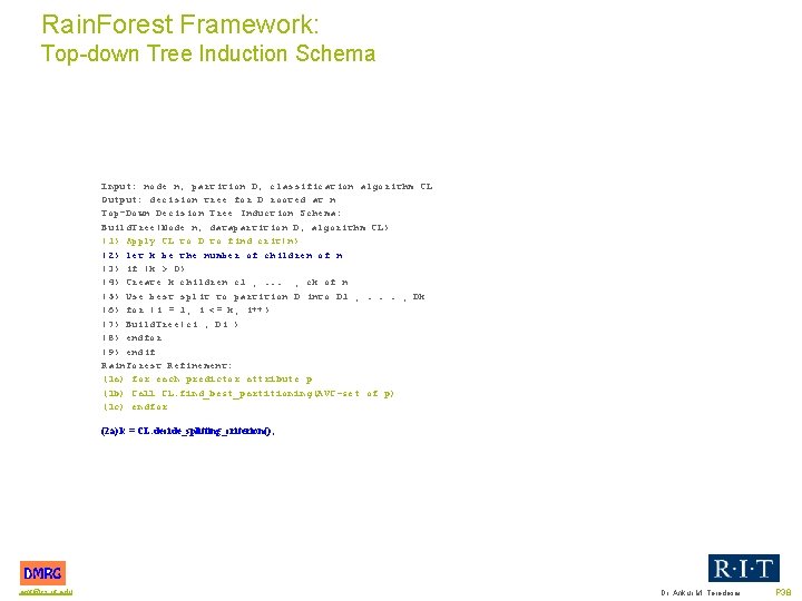
Rain. Forest Framework: Top down Tree Induction Schema Input: node n, partition D, classification algorithm CL Output: decision tree for D rooted at n Top Down Decision Tree Induction Schema: Build. Tree(Node n, datapartition D, algorithm CL) (1) Apply CL to D to find crit(n) (2) let k be the number of children of n (3) if (k > 0) (4) Create k children c 1 ; . . . ; ck of n (5) Use best split to partition D into D 1 ; . . . ; Dk (6) for (i = 1; i <= k; i++) (7) Build. Tree(ci , Di ) (8) endfor (9) endif Rain. Forest Refinement: (1 a) for each predictor attribute p (1 b) Call CL. find_best_partitioning(AVC set of p) (1 c) endfor (2 a) k = CL: decide_splitting_criterion(); amt@cs. rit. edu Dr. Ankur M. Teredesai P 38

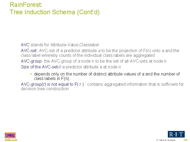
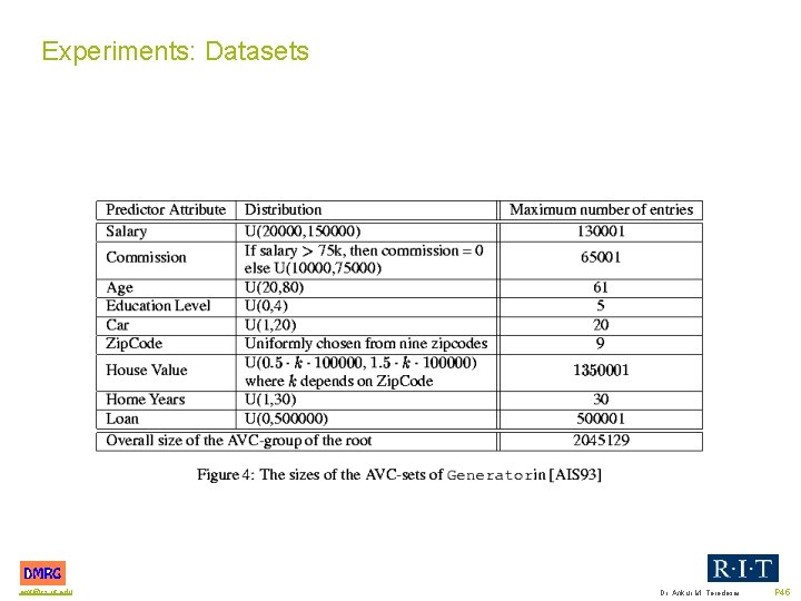
Rain. Forest: Tree Induction Schema (Cont’d) AVC stands for Attribute Value, Classlabel AVC set: AVC set of a predictor attribute a to be the projection of F(n) onto a and the class label whereby counts of the individual class labels are aggregated AVC group: the AVC group of a node n to be the set of all AVC sets at node n. Size of the AVC set of a predictor attribute a at node n • depends only on the number of distinct attribute values of a and the number of class labels in F(n). AVC group(r) is not equal to F( r ) : contains aggregated information that is sufficient for decision tree construction amt@cs. rit. edu Dr. Ankur M. Teredesai P 39

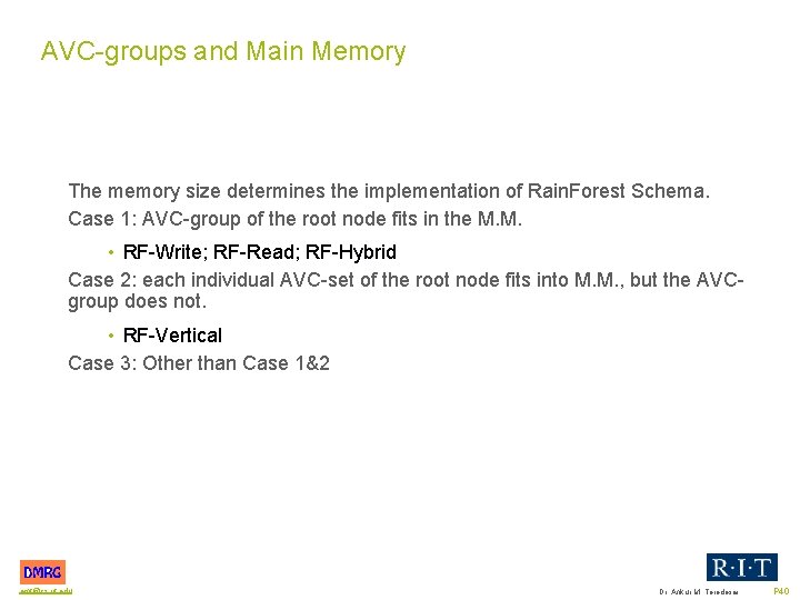
AVC groups and Main Memory The memory size determines the implementation of Rain. Forest Schema. Case 1: AVC group of the root node fits in the M. M. • RF Write; RF Read; RF Hybrid Case 2: each individual AVC set of the root node fits into M. M. , but the AVC group does not. • RF Vertical Case 3: Other than Case 1&2 amt@cs. rit. edu Dr. Ankur M. Teredesai P 40

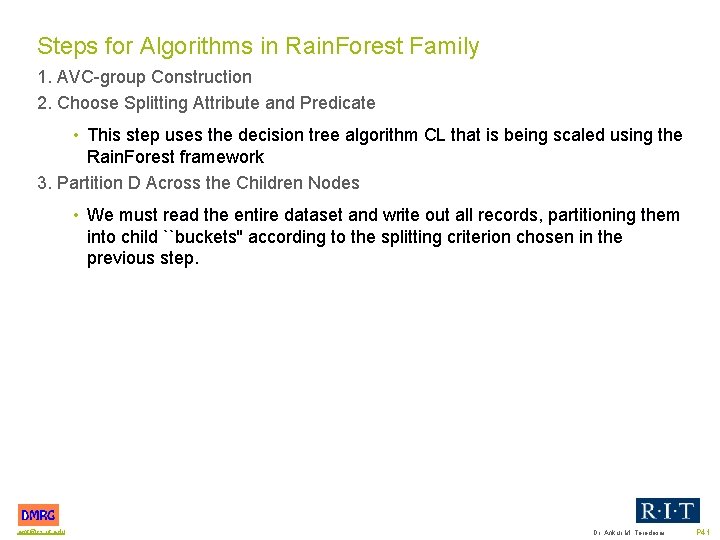
Steps for Algorithms in Rain. Forest Family 1. AVC group Construction 2. Choose Splitting Attribute and Predicate • This step uses the decision tree algorithm CL that is being scaled using the Rain. Forest framework 3. Partition D Across the Children Nodes • We must read the entire dataset and write out all records, partitioning them into child ``buckets'' according to the splitting criterion chosen in the previous step. amt@cs. rit. edu Dr. Ankur M. Teredesai P 41

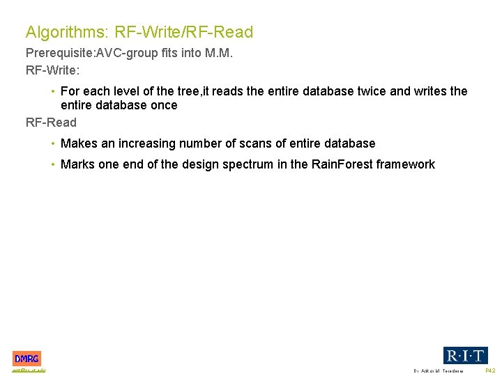
Algorithms: RF Write/RF Read Prerequisite: AVC group fits into M. M. RF Write: • For each level of the tree, it reads the entire database twice and writes the entire database once RF Read • Makes an increasing number of scans of entire database • Marks one end of the design spectrum in the Rain. Forest framework amt@cs. rit. edu Dr. Ankur M. Teredesai P 42

Algorithm: RF Hybrid Combination of RF Write and RF Read Performance can be improved by concurrent construction of AVC sets amt@cs. rit. edu Dr. Ankur M. Teredesai P 43

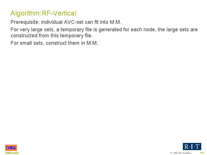
Algorithm: RF Vertical Prerequisite: individual AVC set can fit into M. M. For very large sets, a temporary file is generated for each node, the large sets are constructed from this temporary file. For small sets, construct them in M. M. amt@cs. rit. edu Dr. Ankur M. Teredesai P 44

Experiments: Datasets amt@cs. rit. edu Dr. Ankur M. Teredesai P 45

Experiment Results: (1) When the overall maximum number of entries in the AVC group of the root node is about 2. 1 million, requiring a maximum memory size of 17 MB. amt@cs. rit. edu Dr. Ankur M. Teredesai P 46

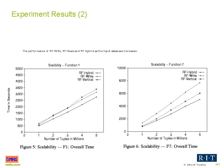
Experiment Results (2) The performance of RF-Write, RF-Read and RF-Hybrid as the input database increases: amt@cs. rit. edu Dr. Ankur M. Teredesai P 47

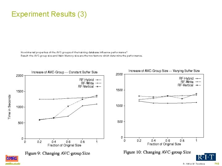
Experiment Results (3) How internal properties of the AVC-groups of the training database influence performance? Result: the AVC-group size and Main Memory size are the two factors which determine the performance. amt@cs. rit. edu Dr. Ankur M. Teredesai P 48

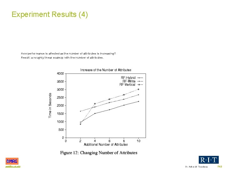
Experiment Results (4) How performance is affected as the number of attributes is increasing? Result: a roughly linear scaleup with the number of attributes. amt@cs. rit. edu Dr. Ankur M. Teredesai P 49

Conclusion A scaling decision tree algorithm that is applicable to all decision tree algorithms at that time. AVC group is the key idea. Database scan at each level of the decision tree Too much dependence over the size of available main memory amt@cs. rit. edu Dr. Ankur M. Teredesai P 50