Decision Trees A divisive method splits Start with
 § Start with “root node” – all")


")


 Open Enterprise Miner File New Project Specify workspace (1)Startup Code")

 Open Enterprise Miner File New Project Specify workspace (1)Startup Code")
 { A A B")


")
 if diversity in parent “node” > summed")
 § Estimates Error Mean")
 can you spare some change? §")
=. 7, Pr(F)=. 3 You say: Sir Ma’am True Gender")


 Hypothetical potency versus chemical content (proportions of A, B, C,")
 Variable Number of Importance Name Splitting Rules B 2. 0")


 p Three Logistic Curves X")

=a+b. X then p = e.")


 3 -0. 4 0. 8 X 1 (-13)")
 Framingham Neural Network Note: No validation data used – surfaces are")

 Use validation data, stop iterating when fit gets worse")


 item cart bread 1 milk 1 soap 2 meat")

 § We do NOT have the")
 Plot clusters and actual target values:")

 : release 1: Did the NCAA")


 agrees ! Cluster 2 Cluster 1")
 Usual name: Nearest Neighbor Analysis Probe Point 9 blue 7")

 scored by Enterprise Miner Nearest Neighbor method Original Data scored by")
 Assumes multivariate normal")
 Three Populations: (pay all credit card debt, pay")


/9 when variance was 9 in every")


- Slides: 89
Decision Trees § A “divisive” method (splits) § Start with “root node” – all in one group § Get splitting rules § Response often binary § Result is a “tree” § Example: Loan Defaults § Example: Framingham Heart Study § Example: Automobile Accidentsnts
Recursive Splitting Pr{default} =0. 008 Pr{default} =0. 012 Pr{default} =0. 006 X 1=Debt To Income Ratio Pr{default} =0. 0001 Pr{default} =0. 003 No default Default X 2 = Age
Some Actual Data § Framingham Heart Study § First Stage Coronary Heart Disease § P{CHD} = Function of: » Age - no drug yet! » Cholesterol » Systolic BP Import
Example of a “tree” Using Default Settings
Example of a “tree” Using Custom Settings (Gini splits, N=4 leaves)
How to make splits? § Contingency tables Heart Disease No Yes 180 ? 240? Low BP High BP Heart Disease No Yes 95 5 100 55 45 100 150 50 DEPENDENT (effect) 75 75 25 25 100 150 50 INDEPENDENT (no effect)
How to make splits? § Contingency tables Heart Disease No Yes 180 ? 240? Low BP High BP 95 75 5 25 45 25 150 50 DEPENDENT (effect) Observed - Expected 100 Expected 2(400/75)+ 2(400/25) = 42. 67 Compare to c 2 tables – Significant! (Why do we say “Significant” ? ? ? ) =
H 0 : H 1 : H 0: Innocence H 1: Guilt 95 75 5 25 H 0: No association H 1: BP and heart disease are associated 55 75 45 25 P=0. 0000064 Beyond reasonable doubt P<0. 05 Framingham Conclusion: Sufficient evidence against the (null) hypothesis of no relationship.
Demo 1: Chi-Square for Titanic Survival (S Crew 3 rd Class 2 nd Class 1 st Class Alive 212 178 118 202 Dead 696 528 167 123 all possible splits c 2 Crew vs. other 51. 94 Crew&3 versus 1&2 163. 09 First versus other 160. 04 “logworth” = P-value -log 10(p-value) 5. 7 x 10 -13 12. 24 2. 4 x 10 -37 36. 62 1. 1 x 10 -36 35. 96
Demo 2: Titanic (EM) Open Enterprise Miner File New Project Specify workspace (1)Startup Code – specify data library (2)New Data Source Titanic (3)Data has class (1, 2, 3, crew) & MWC (4)Bring in data, Decision Tree (defaults)
3 possible splits for M, W, C 10 possible splits for class (is that fair? )
Demo 3: Framingham (EM) Open Enterprise Miner File New Project Specify workspace (1)Startup Code – specify data library (2)New Data Source Framingham (a)Firstchd = target, reject obs (b)Explore Firschd (pie) vs. Age (histogram) (3)Bring in data, Decision Tree (defaults)
Other Sp lit Criteria § Gini Diversity Index § (1) { A A B A B B C B} § Pick 2, Pr{different} = 1 -Pr{AA}-Pr{BB}-Pr{CC} » 1 -. 25 -. 16 -. 01=. 58 (sampling with replacement) § (2) { A A B C B A A B C C } » 1 -. 16 -. 09= 0. 66 group (2) is more diverse (less pure) § Shannon Entropy § Larger more diverse (less pure) § -Si pi log 2(pi) {0. 5, 0. 4, 0. 1} 1. 36 {0. 4, 0. 2, 0. 3} 1. 51 (more diverse)
How to make splits? § Which variable to use? § Where to split? § Cholesterol > ____ § Systolic BP > _____ § Idea – Pick BP cutoff to minimize p-value for c 2 § Split point data-derived! § What does “significance” mean now?
Multiple testing a = Pr{ falsely reject hypothesis 2} a a a = Pr{ falsely reject hypothesis 1} Pr{ falsely reject one or the other} < 2 a Desired: 0. 05 probability or less Solution: Compare 2(p-value) to 0. 05
Validatio n § Traditional stats – small dataset, need all observations to estimate parameters of interest. § Data mining – loads of data, can afford “holdout sample” § Variation: n-fold cross validation § § Randomly divide data into n sets Estimate on n-1, validate on 1 Repeat n times, using each set as holdout. Titanic and Framingham examples did not use holdout.
Prunin g § Grow bushy tree on the “fit data” § Classify validation (holdout) data § Likely farthest out branches do not improve, possibly hurt fit on validation data § Prune non-helpful branches. § What is “helpful”? What is good discriminator criterion?
Goal s § Split (or keep split) if diversity in parent “node” > summed diversities in child nodes § Prune to optimize § Estimates § Decisions § Ranking § in validation data
§ Assessment for: Decisions Minimize incorrect decisions (model versus realized) § Estimates Error Mean Square (average error) § Ranking C (concordance) statistic = proportion concordant + ½ (proportion tied) § Obs number 1 (2, 3) 4 5 § Probability of 0 0. 2 0. 3 0. 6 0. 7 ( from model) § Actual 0 (0, 1) 1 0 » Concordant Pairs: (1, 3) (1, 4) (2, 4) » Discordant Pairs: (3, 5) (4, 5) » Tied (2, 3) » 6 ways to get pair with 2 different responses § C = 3/6 + (1/2)(1/6) = 7/12=0. 5833
Accounting for Costs § Pardon me (sir, ma’am) can you spare some change? § Say “sir” to male +$2. 00 § Say “ma’am” to female +$5. 00 § Say “sir” to female -$1. 00 (balm for slapped face) § Say “ma’am” to male -$10. 00 (nose splint)
Including Probabilities Leaf has Pr(M)=. 7, Pr(F)=. 3 You say: Sir Ma’am True Gender M F 0. 7 (2) 0. 3 (-1) 0. 7 (-10) 0. 3 (5) +$1. 10 -$5. 50 Expected profit is 2(0. 7)-1(0. 3) = $1. 10 if I say “sir” Expected profit is -7+1. 5 = -$5. 50 (a loss) if I say “Ma’am” Weight leaf profits by leaf size (# obsns. ) and sum. Prune (and split) to maximize profits.
Regression Trees § Continuous response Y § Predicted response Pi constant in regions i=1, …, 5 Predict 80 Predict 50 X 2 Predict 130 Predict 100 X 1 Predict 20
Regression Trees § Predict Pi in cell i. § Yij jth response in cell i. § Split to minimize Si Sj (Yij-Pi)2
Real data example: Traffic accidents in Portugal* Y = injury induced “cost to society” Help - I ran Into a “tree” * Tree developed by Guilhermina Torrao, (used with permission) NCSU Institute for Transportation Research & Education Help - I ran Into a “tree”
Demo 4: Chemicals (EM) Hypothetical potency versus chemical content (proportions of A, B, C, D) New Data Source Chemicals {Sum, Dead} rejected, Potency Target, Partition node: training 75%, validation 25% Connect and run tree node, look at results Tree Node, Results. View Model Variable Importance
Demo 4 (cont. ) Variable Number of Importance Name Splitting Rules B 2. 0 1. 0 A 4. 0 0. 68 C 0. 0 D 0. 0 Validation Ratio of Validation Importance to Training Importance 1. 0 0. 63 0. 94 0. 0 Na. N Only A and B amounts contribute to splits. B splits reduce variation more. A reduces it by about 2/3 as much as B. Properties panel Exported data Explore 3 D graph X=A Y=B Z=P_Potency
B A A A B A
3 5 1 6 2 4
Logistic Regression § Logistic – another classifier § Older – “tried & true” method § Predict probability of response from input variables (“Features”) § Linear regression gives infinite range of predictions § 0 < probability < 1 so not linear regression.
Logistic Regression ea+b. X (1+ea+b. X) p Three Logistic Curves X
Example: Seat Fabric Ignition § Flame exposure time = X § Y=1 ignited, Y=0 did not ignite § Y=0, X= 3, 5, 9 10 , 13, 16 § Y=1, X = 7 11, 12 14, 15, 17, 25, 30 § Q=(1 -p 1)(1 -p 2)(1 -p 3)(1 -p 4)p 5 p 6(1 -p 7)p 8 p 9(1 -p 10)p 11 p 12 p 13 § p’s all different pi = f(a+b. Xi) = ea+b. Xi/(1+ea+b. Xi) § Find a, b to maximize Q(a, b)
§ Logistic idea: § Given temperature X, compute L(x)=a+b. X then p = e. L/(1+e. L) maximize Q(a, b) § p(i) = ea+b. Xi/(1+ea+b. Xi) § Write p(i) if response, 1 -p(i) if not § Multiply all n of these together, find a, b to maximize this “likelihood” § Estimated L = ___+ ____X -2. 6 a b 0. 23
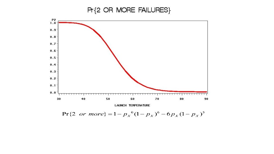
Example: Shuttle Missions § O-rings failed in Challenger disaster § Prior flights “erosion” and “blowby” in O-rings (6 per mission) § Feature: Temperature at liftoff § Target: (1) - erosion or blowby vs. no problem (0) L=5. 0850 – 0. 1156(temperature) p = e. L/(1+e. L)
Neural Networks X 1 inputs X 2 § Very flexible functions X 3 § “Hidden Layers” X 4 § “Multilayer Perceptron” H 1 (0, 1) Output = Pr{1} H 2 Logistic function of Logistic functions ** Of data ** (note: Hyperbolic tangent functions are just reparameterized logistic functions)
Example: Y = a + b 1 H 1 + b 2 H 2 + b 3 H 3 Y = 0 + 9 H 1 + 3 H 2 + 5 H 3 “bias” -1 to 1 “weights” H 1 X H 2 b 1 b 2 Y b 3 H 3 Arrows on right represent linear combinations of “basis functions, ” e. g. hyperbolic tangents (reparameterized logistic curves)
A Complex Neural Network Surface (-10) 3 -0. 4 0. 8 X 1 (-13) 0 -1 0. 25 X 2 -0. 9 0. 01 (20) (“biases”) 2. 5 (-1) P
Demo 5 (EM) Framingham Neural Network Note: No validation data used – surfaces are unnecessarily complex . 001 Sbp 200 -10 0 Ch 13 ole 0 - st 28 0 . 057 Age 25 Smoker. 057 Sbp 200 -100 Ch 13 ole 0 - st 28 0 Age 25 Nonsmoker “Slice” of 4 -D surface at age=25 Code for graphs in NNFramingham. sas
Framingham Neural Network Surfaces “Slice” at age 55 – are these patterns real? Age 55 Nonsmoker . 261 . 009 . 004 Sbp 200 -10 Ch 13 ole 0 - st 28 0 . 262 0 Sbp 200 -100 Ch 13 ole 0 - st 28 0 Age 55 Smoker
Handling Neural Net Complexity (1) Use validation data, stop iterating when fit gets worse on validation data. Problems for Framingham (50 -50 split) Fit gets worse at step 1 no effect of inputs. Algorithm fails to converge (likely reason: too many parameters) (2) Use regression to omit predictor variables (“features”) and their parameters. This gives previous graphs. (3) Do both (1) and (2). 41
Lift 3. 3 * Cumulative Lift Chart - Go from leaf of most to least predicted response. - Lift is proportion responding in first p% 1 overall population response rate Predicted response high ------------------- low
Receiver Operating Characteristic Curve Cut point 1 Logits of 1 s Logits of 0 s red black (or any model predictor from most to least likely to respond) Select most likely p 1% according to model. Call these 1, the rest 0. (call almost everything 0) Y=proportion of all 1’s correctly identified. (Y near 0) X=proportion of all 0’s incorrectly called 1’s (X near 0)
Receiver Operating Characteristic Curve Cut point 2 Logits of 1 s Logits of 0 s red black Select most likely p 2% according to model. Call these 1, the rest 0. Y=proportion of all 1’s correctly identified. X=proportion of all 0’s incorrectly called 1’s
Receiver Operating Characteristic Curve Cut point 3 Logits of 1 s Logits of 0 s red black Select most likely p 3% according to model. Call these 1, the rest 0. Y=proportion of all 1’s correctly identified. X=proportion of all 0’s incorrectly called 1’s
Receiver Operating Characteristic Curve Cut point 3. 5 Logits of 1 s Logits of 0 s red black Select most likely 50% according to model. Call these 1, the rest 0. Y=proportion of all 1’s correctly identified. X=proportion of all 0’s incorrectly called 1’s
Receiver Operating Characteristic Curve Cut point 4 Logits of 1 s Logits of 0 s red black Select most likely p 5% according to model. Call these 1, the rest 0. Y=proportion of all 1’s correctly identified. X=proportion of all 0’s incorrectly called 1’s
Receiver Operating Characteristic Curve Cut point 5 Logits of 1 s Logits of 0 s red black Select most likely p 6% according to model. Call these 1, the rest 0. Y=proportion of all 1’s correctly identified. X=proportion of all 0’s incorrectly called 1’s
Receiver Operating Characteristic Curve Cut point 6 Logits of 1 s Logits of 0 s red black Select most likely p 7% according to model. Call these 1, the rest 0. (call almost everything 1) Y=proportion of all 1’s correctly identified. (Y near 1) X=proportion of all 0’s incorrectly called 1’s (X near 1)
Why is area under the curve the same as number of concordant pairs + (number of ties)/2 ? ? Tree Leaf 1: 20 0’s, 60 1’s Leaf 2: 20 0’s, 20 1’s Leaf 3: 60 0’s 20 1’s Cut pt. 0 1 2 3 Left of cut, call it 1 | and right of cut, call it 0. X = number of incorrect 0 decisions , Y= number of correct 1 decisions X = number of 0’s to the left of cut point, Y = number of 1’s to the left of cut point. (X, Y) on ROC curve Cut 0 X=0 (all points called 0 so none wrong) Y=0 (no 1 decisions) (0, 0) Cut 1 (20)(60) = 1200 ties, 60(20+60)=1200 concordant (20, 60) 60 1’s (0, 0) 20 60 Ties Concordant Areas are number of tied pairs in leaf 1 plus number of concordant pairs from 0’s in leaves 2 and 3 ROC curve (line) splits ties in two.
Why is area under the curve the same as number of concordant pairs + (number of ties)/2? ? Tree Leaf 1: 20 0’s, 60 1’s Leaf 2: 20 0’s, 20 1’s Leaf 3: 60 0’s 20 1’s Cut pt. 0 1 2 3 Left of cut, call it 1 | and right of cut, call it 0. Cut point 2: 20 more 1’s, 60 0’s to the right, 20 x 20=400 ties in leaf 2. point on ROC curve: (40. 80) Cut point 3: call everything a 1. All 100 1’s are correctly called, all 0’s incorrectly called. point on ROC curve: (100, 100) 20 1’s ROC curve is in terms of proportions so join points are (0, 0), (. 2, . 6), (. 4, . 8), and (1, 1). For Logistic Regression or Neural Nets, each point is a potential cut point for the ROC curve. 60 1’s (1, 1) ----(0. 4, 0. 8) 20 60 0’s -(0. 2, 0. 6) Ties Concordant (0, 0)
Framingham ROC for 4 models and baseline 45 degree line Neural net highlighted, area 0. 780 Sensitivity: Pr{ calling a 1 }=Y coordinate Specificity; Pr{ calling a 0 } = 1 -X. Selected Model Node Model Description Misclassification Rate Avg. Squared Area Under Error ROC Y Neural Network 0. 079257 0. 066890 0. 780 Tree Decision Tree 0. 079257 0. 069369 0. 720 Tree 2 Gini Tree N=4 0. 079257 0. 675 Regression 0. 080495 0. 069604 52 0. 069779 0. 734
A Combined Example Cell Phone Texting Locations Black circle: Phone moved > 50 feet in first two minutes of texting. Green dot: Phone moved < 50 feet. .
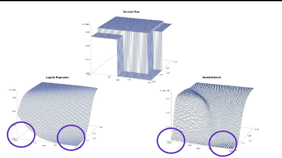
Tree Neural Net Logistic Regression Three Models Training Data Lift Charts Validation Data Lift Charts Resulting Surfaces
Demo 5: Three Breast Cancer Models Features are computed from a digitized image of a fine needle aspirate (FNA) of a breast mass. They describe characteristics of the cell nuclei present in the image. 1. Sample code number id number 2. Clump Thickness 1 - 10 3. Uniformity of Cell Size 1 - 10 4. Uniformity of Cell Shape 1 - 10 5. Marginal Adhesion 1 - 10 6. Single Epithelial Cell Size 1 - 10 7. Bare Nuclei 1 - 10 8. Bland Chromatin 1 - 10 9. Normal Nucleoli 1 - 10 10. Mitoses 1 - 10 11. Class: (2 for benign, 4 for malignant)
Use Decision Tree to Pick Variables
Decision Tree Needs Only BARE & SIZE
Can save scoring code from EM Data A; do bare=0 to 10; do size=0 to 10; (score code from EM) Output; end; M o d e l C o m p a r i s o n N o d e R e s u l t s Cancer Screening Results: Model Comparison Node Selected Model Node Model Description Train Avg. Train Area Misclassification Squared Under ROC Rate Error Validation Misclassification Rate Validation Avg. Area Under Squared Error ROC Y Tree Decision Tree 0. 031429 0. 029342 0. 975 0. 051576 0. 048903 0. 933 Neural Network 0. 031429 0. 025755 0. 994 0. 054441 0. 037838 0. 985 Regression 0. 031429 0. 029322 0. 992 0. 054441 0. 040768 0. 987
Association Analysis is just elementary probability with new names 0. 3 A Pr{A and B} Pr{A} =0. 5 = 0. 2 Pr{B} =0. 3 A: Purchase Milk B B: Purchase Cereal 0. 1 0. 4 0. 3+0. 2+0. 1+0. 4 = 1. 0
Cereal=> Milk Rule B=> A “people who buy B will buy A” Support: Support= Pr{A and B} = 0. 2 A 0. 3 B 0. 2 0. 1 0. 4 Independence means that Pr{A|B} = Pr{A} = 0. 5 = Expected confidence if there is no relation to B. . Confidence: Confidence = Pr{A|B}=Pr{A and B}/Pr{B}=2/3 ? ? - Is the confidence in B=>A the same as the confidence in A=>B? ? (yes, no) Lift: Lift = confidence / E{confidence} = (2/3) / (1/2) = 1. 33 Gain = 33% B Marketing A to the 30% of people who buy B will result in 33% better sales than marketing to a random 30% of the people.
Example: Grocery cart items (hypothetical) item cart bread 1 milk 1 soap 2 meat 3 bread 4 cereal 4 milk 4 soup 5 bread 5 cereal 5 milk 5 Sort Criterion: Confidence Maximum Items: 2 Minimum (single item) Support: 20% Association Report Expected Confidence Support Transaction Relations (%) Lift Count Rule 2 63. 43 84. 21 52. 68 1. 33 8605 cereal ==> milk 2 62. 56 83. 06 52. 68 1. 33 8605 milk ==> cereal 2 63. 43 61. 73 12. 86 0. 97 2100 meat ==> milk 2 63. 43 61. 28 38. 32 0. 97 6260 bread ==> milk 2 63. 43 60. 77 12. 81 0. 96 2093 soup ==> milk 2 62. 54 60. 42 38. 32 0. 97 6260 milk ==> bread 2 62. 56 60. 28 37. 70 0. 96 6158 bread ==> cereal 2 62. 54 60. 26 37. 70 0. 96 6158 cereal ==> bread 2 62. 56 60. 16 12. 69 0. 96 2072 soup ==> cereal 2 21. 08 20. 28 12. 69 0. 96 2072 cereal ==> soup 2 20. 83 20. 27 12. 86 0. 97 2100 milk ==> meat 2 21. 08 20. 20 12. 81 0. 96 2093 milk ==> soup
Link Graph Sort Criterion: Confidence Maximum Items: 3 e. g. milk & cereal bread Minimum Support: 5% Slider bar at 62%
Unsupervised Learning § We have the “features” (predictors) § We do NOT have the response even on a training data set (UNsupervised) § Another name for clustering § EM § Large number of clusters with k-means (k clusters) § Ward’s method to combine (less clusters , say r<k) § One more k means for final r-cluster solution.
Example: Cluster the breast cancer data (disregard target) Plot clusters and actual target values:
Segment Profiler
Text Mining Hypothetical collection of news releases (“corpus”) : release 1: Did the NCAA investigate the basketball scores and vote for sanctions? release 2: Republicans voted for and Democrats voted against it for the win. (etc. ) Compute word counts: NCAA basketball score vote Republican Democrat win Release 1 1 1 0 0 Release 2 0 0 2 1 1
Text Mining Mini-Example: Word counts in 16 e-mails ----------------words--------------------- R B P e a r p s e u k s b e i l t d i b e c a n a l t n l d o c u m e n t E l e c t i o n 1 2 3 4 5 6 7 8 9 10 11 12 13 14 20 5 0 8 0 10 2 4 26 19 2 16 14 1 T o D u e r S S m V n S c c o o a p o o c t N L m e W r r r e C i e e a r A a n c n _ _ t s A r t h s V N 8 10 12 6 0 1 5 3 8 18 15 21 6 9 5 4 2 0 9 0 12 12 9 0 2 0 14 0 2 12 0 16 4 24 19 30 9 7 0 12 14 2 12 3 15 22 8 2 0 4 16 0 0 15 2 17 3 9 0 1 6 9 5 5 19 5 20 0 18 13 9 14 3 1 13 0 1 12 13 20 0 0 1 6 1 4 16 2 4 9 0 12 9 3 0 0 13 9 2 16 20 6 24 4 30 9 10 14 22 10 11 9 12 0 14 10 22 3 1 0 0 0 14 1 3 12 0 16 12 17 23 8 19 21 0 13 9 0 16 4 12 0 0 2 17 12 0 20 19 0 12 5 9 6 1 4 0 4 21 3 6 9 3 8 0 3 10 20
Eigenvalues of the Correlation Matrix Eigenvalue 1 2 3 4 5 7. 10954264 2. 30455155 1. 00292318 0. 76887967 0. 55817886 13 0. 0008758 Difference Proportion 4. 80499109 1. 30162837 0. 23404351 0. 21070080 0. 10084923 (more) Variable Prin 1 Cumulative 0. 5469 0. 1773 0. 0771 0. 0591 0. 0429 0. 5469 0. 7242 0. 8013 0. 8605 0. 9034 0. 0001 1. 0000 55% of the variation in these 13 -dimensional vectors occurs in one dimension. Prin 2 Prin 1 Basketball -. 320074 NCAA -. 314093 Tournament -. 277484 Score_V -. 134625 Score_N -. 120083 Wins -. 080110 Speech 0. 273525 Voters 0. 294129 Liar 0. 309145 Election 0. 315647 Republican 0. 318973 President 0. 333439 Democrat 0. 336873
Eigenvalues of the Correlation Matrix Eigenvalue 1 2 3 4 5 7. 10954264 2. 30455155 1. 00292318 0. 76887967 0. 55817886 13 0. 0008758 Difference 4. 80499109 1. 30162837 0. 23404351 0. 21070080 0. 10084923 (more) Proportion Variable Prin 1 Cumulative 0. 5469 0. 1773 0. 0771 0. 0591 0. 0429 0. 5469 0. 7242 0. 8013 0. 8605 0. 9034 0. 0001 1. 0000 Prin 2 Prin 1 55% of the variation in these 13 -dimensional vectors occurs in one dimension. Basketball -. 320074 NCAA -. 314093 Tournament -. 277484 Score_V -. 134625 Score_N -. 120083 Wins -. 080110 Speech 0. 273525 Voters 0. 294129 Liar 0. 309145 Election 0. 315647 Republican 0. 318973 President 0. 333439 Democrat 0. 336873
Sports Cluster Politics Cluster
d o C c L u U m S e T n E t R R B T P e a o E r p s D u l e u k e r S S e s b e m V n S c c P c. P i l t o o a p o o r tr d i b c t N L m e W r r i i ie c a r e C i e e n on n a l a r A a n c n _ _ 1 n 1 t n l t s A r t h s V N 3 1 -3. 63815 11 1 -3. 02803 Sports 5 1 -2. 98347 Documents 14 1 -2. 48381 7 1 -2. 37638 8 1 -1. 79370 0 2 0 14 0 2 12 0 16 4 24 19 30 2 0 0 14 1 3 12 0 16 12 17 23 8 0 0 4 16 0 0 15 2 17 3 9 0 1 1 0 4 21 3 6 9 3 8 0 3 10 20 2 3 1 13 0 1 12 13 20 0 0 1 6 4 1 4 16 2 4 9 0 12 9 3 0 0 (biggest gap) 1 2 -0. 00738 20 8 10 12 6 0 1 5 3 8 18 15 21 2 2 0. 48514 5 6 9 5 4 2 0 9 0 12 12 9 0 Politics 6 2 1. 54559 10 6 9 5 5 19 5 20 0 18 13 9 14 Documents 4 2 1. 59833 8 9 7 0 12 14 2 12 3 15 22 8 2 10 2 2. 49069 19 22 10 11 9 12 0 14 10 22 3 1 0 13 2 3. 16620 14 17 12 0 20 19 0 12 5 9 6 1 4 12 2 3. 48420 16 19 21 0 13 9 0 16 4 12 0 0 2 9 2 3. 54077 26 13 9 2 16 20 6 24 4 30 9 10 14
PROC CLUSTER (single linkage) agrees ! Cluster 2 Cluster 1
Memory Based Reasoning (optional) Usual name: Nearest Neighbor Analysis Probe Point 9 blue 7 red Classify as BLUE Estimate Pr{Blue} as 9/16
Note: Enterprise Miner Exported Data Explorer Chooses colors
Score Data (grid) scored by Enterprise Miner Nearest Neighbor method Original Data scored by Enterprise Miner Nearest Neighbor method
Fisher’s Linear Discriminant Analysis - an older method of classification (optional) Assumes multivariate normal distribution of inputs (features) Computes a “posterior probability” for each of several classes, given the observations. Based on statistical theory
Example: One input, (financial stress index) Three Populations: (pay all credit card debt, pay part, default). Normal distributions with same variance. Classify a credit card holder by financial stress index: pay all (stress<20), pay part (20<stress<27. 5), default(stress>27. 5) Data are hypothetical. Means are 15, 25, 30.
Example: Differing variances. Not just closest mean now. Normal distributions with different variances. Classify a credit card holder by financial stress index: pay all (stress<19. 48), pay part (19. 48<stress<26. 40), default(26. 40<stress<36. 93), pay part (stress>36. 93) Data are hypothetical. Means are 15, 25, 30. Standard Deviations 3, 6, 3.
Example: 20% defaulters, 40% pay part 40% pay all Normal distributions with same variance and “priors. ” Classify a credit card holder by financial stress index: pay all (stress<19. 48), pay part (19. 48<stress<28. 33), default(28. 33<stress<35. 00), pay part (stress>35. 00) Data are hypothetical. Means are 15, 25, 30. Standard Deviations 3, 6, 3. Population size ratios 2: 2: 1
m = 15, 25, or 30, s =3 here. The part that changes from one population to another is Fisher’s linear discriminant function. Here it is (mx-m 2/2)/s 2, that is, (mx-m 2/2)/9. The bigger this is, the more likely it is that X came from the population with mean m. The three probability densities are in the same proportions as their values of exp((mx-m 2/2)/9).
Example: Stress index X=21. Classify as someone that pays only part of credit card bill because 21 is closer to 25 than to 15 or 30. Probabilities 0. 24, 0. 74, 0. 02 give more detail. m = 15, 25, or 30, s =here. 15 25 30 22. 5 23. 61 20. 00 59. 11*108 179. 5*108 4. 85*108 probability 0. 24 0. 74 0. 02
Fisher for credit card data was (mx-m 2/2)/9 when variance was 9 in every group. (mx-m 2/2)/9 = 1. 67 X-12. 50 for mean 15 (mx-m 2/2)/9 = 1. 67 X-34. 72 for mean 25 (mx-m 2/2)/9 = 1. 67 X-50. 00 for mean 30 For 2 inputs it again has a linear form ___+___X 1+___X 2 where the coefficients come from the bivariate mean vector and the 2 x 2 matrix is assumed constant across populations. When variances differ, formulas become more complicated, discriminant becomes quadratic, and boundaries are not linear.
Example: Two inputs, three populations Multivariate normals, same 2 x 2 covariance matrix. Viewed from above, boundaries appear to be linear.
Defaults Pays part only debt Pays in full Income
Generated sample: 1000 per group Debt index Income index
proc discrim data=a; class group; var X 1 X 2; run; _ -1 _ -1 _ Constant = -. 5 X' COV X Coefficient Vector = COV X j j Linear Discriminant Function for group Variable 1 2 3 Constant -20. 09529 -0. 31096 -1. 73324 X 1 -1. 91229 0. 12222 -0. 06775 X 2 2. 13365 0. 19059 -0. 61763
Number of Observations and Percent Classified into group From group 1 2 3 Total 1000 0 0 1000 100. 00 100. 00 2 0 907 93 1000 0. 00 90. 70 9. 30 100. 00 3 0 112 888 1000 0. 00 11. 20 88. 80 100. 00 Total 1000 1019 981 3000 33. 33 33. 97 32. 70 100. 00 Priors 0. 33333 Error Count Estimates for group 1 2 3 Total Rate 0. 0000 0. 0930 0. 1120 0. 0683 Priors 0. 3333
Generated sample: 1000 per group Sample Discriminants Differ Somewhat from Theoretical Defaults Debt index Pays part only Pays in full Income index