Decision Trees 3 Example 1 Iris v Datasets


 함수: Decision Tree를 생성하는 함수 8")


 v 다른 속성과 type간의 관계를 box plot으로 표현 –")
 17")


- Slides: 22
Decision Trees 3
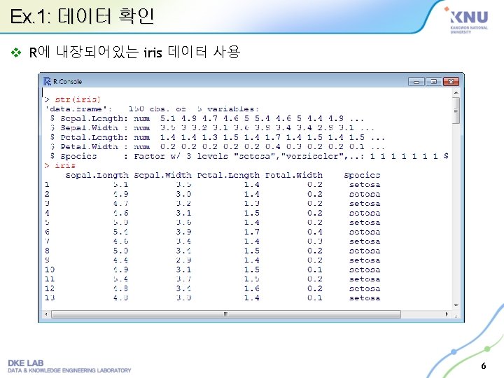
Example 1: Iris v Datasets: 150개의 Iris 꽃 데이터 – Sepal. Length: 꽃 받침 길이 – Sepal. Width: 꽃 받침 너비 – Petal. Length: 꽃잎 길이 – Petal. Width: 꽃잎 너비 – Species: 화종 • setosa • versicolor • virginica # Sepal. Length Sepal. Width Petal. Length Petal. Width Species 1 5. 1 3. 5 1. 4 0. 2 setosa 2 4. 9 3 1. 4 0. 2 setosa 3 4. 7 3. 2 1. 3 0. 2 setosa 4 4. 6 3. 1 1. 5 0. 2 setosa 5 5 3. 6 1. 4 0. 2 setosa 6 5. 4 3. 9 1. 7 0. 4 setosa 7 4. 6 3. 4 1. 4 0. 3 setosa 8 5 3. 4 1. 5 0. 2 setosa 9 4. 4 2. 9 1. 4 0. 2 setosa 10 4. 9 3. 1 1. 5 0. 1 setosa 11 5. 4 3. 7 1. 5 0. 2 setosa 12 4. 8 3. 4 1. 6 0. 2 setosa 13 4. 8 3 1. 4 0. 1 setosa 14 4. 3 3 1. 1 0. 1 setosa 15 5. 8 4 1. 2 0. 2 setosa 새로운 Iris 데이터의 종을 파악할 수 있을까? 4
Ex. 1: 필수 패키지 설치 v Decision Tree를 생성하기 위해 필요한 패키지 설치 – http: //cran. r-project. org/web/packages/party/index. html – http: //cran. r-project. org/web/packages/zoo/index. html – http: //cran. r-project. org/web/packages/sandwich/index. html – http: //cran. r-project. org/web/packages/strucchange/index. html – http: //cran. r-project. org/web/packages/modeltools/index. html – http: //cran. r-project. org/web/packages/coin/index. html – http: //cran. r-project. org/web/packages/mvtnorm/index. html v 다운로드 받은 패키지를 R에서 로딩 5
Ex. 1: Decision Tree 생성 v ctree() 함수: Decision Tree를 생성하는 함수 8
Ex. 1: Decision Tree 생성 v Decision Tree 플로팅 9
Ex. 1: Decision Tree 생성 v Decision Tree 플로팅 10
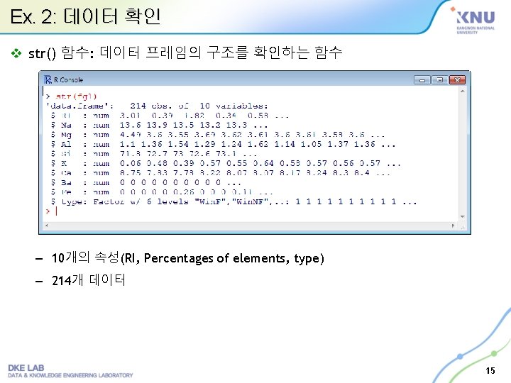
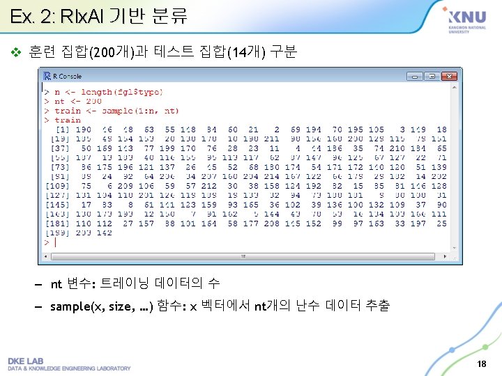
Example 2: Forensic Glass v Datasets: 6 종류의 유리조각 214개 데이터 – Win. F: float glass window # RI Na Mg – Win. NF: non-float glass window 1 3. 01 13. 64 4. 49 2 -0. 39 13. 89 3 -1. 82 – Con: container (bottles) 4 – Tabl: Tableware – Head: vehicle headlamp – Veh: vehicle window v 각 데이터는 다음의 속성을 가짐 – RI: 굴절률(refractive index) Al Si K Ca Ba Fe type 1. 1 71. 78 0. 06 8. 75 0 0 Win. F 3. 6 1. 36 72. 73 0. 48 7. 83 0 0 Win. F 13. 53 3. 55 1. 54 72. 99 0. 39 7. 78 0 0 Win. F -0. 34 13. 21 3. 69 1. 29 72. 61 0. 57 8. 22 0 0 Win. F 5 -0. 58 13. 27 3. 62 1. 24 73. 08 0. 55 8. 07 0 0 Win. F 6 -2. 04 12. 79 3. 61 1. 62 72. 97 0. 64 8. 07 0 0. 26 Win. F 7 -0. 57 13. 3 3. 6 1. 14 73. 09 0. 58 8. 17 0 0 Win. F 8 -0. 44 13. 15 3. 61 1. 05 73. 24 0. 57 8. 24 0 0 Win. F 9 1. 18 14. 04 3. 58 1. 37 72. 08 0. 56 8. 3 0 0 Win. F – Percentages of Na, Mg, Al, Si, K, Ca, Ba, and Fe – type: 유리의 종류 새로운 유리조각의 종류를 파악할 수 있을까? 13
Ex. 2: 필수 패키지 설치 v 데이터 셋을 수집하기 위해, 관련 패키지 다운로드 – http: //cran. r-project. org/web/packages/textir/index. html – http: //cran. r-project. org/web/packages/distrom/index. html – http: //cran. r-project. org/web/packages/gamlr/index. html – 압축 해제 후, 설치 경로의 library 폴더로 이동 v 다운로드 받은 패키지를 R에서 로딩 14
Ex. 2: Box plots (1/2) v 다른 속성과 type간의 관계를 box plot으로 표현 – par() 함수: 그래프의 공간을 배열 형태로 미리 할당 › par(mfrow=c(3, 3), mai=c(. 3, . 6, . 1)) › plot(RI ~ type, data=fgl, col=c(grey(. 2), 2: 6)) › plot(Al ~ type, data=fgl, col=c(grey(. 2), 2: 6)) › plot(Na ~ type, data=fgl, col=c(grey(. 2), 2: 6)) › plot(Mg ~ type, data=fgl, col=c(grey(. 2), 2: 6)) › plot(Ba ~ type, data=fgl, col=c(grey(. 2), 2: 6)) › plot(Si ~ type, data=fgl, col=c(grey(. 2), 2: 6)) › plot(K ~ type, data=fgl, col=c(grey(. 2), 2: 6)) › plot(Ca ~ type, data=fgl, col=c(grey(. 2), 2: 6)) › plot(Fe ~ type, data=fgl, col=c(grey(. 2), 2: 6)) 16
Ex. 2: Box plots (2/2) 17