Decision Trees 2 Numerical attributes Tests in nodes

Decision Trees (2)

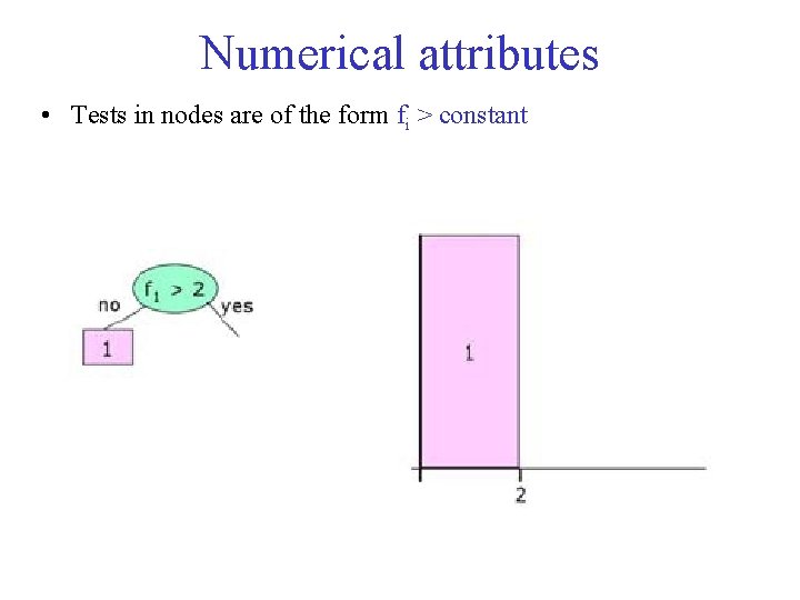
Numerical attributes • Tests in nodes are of the form fi > constant

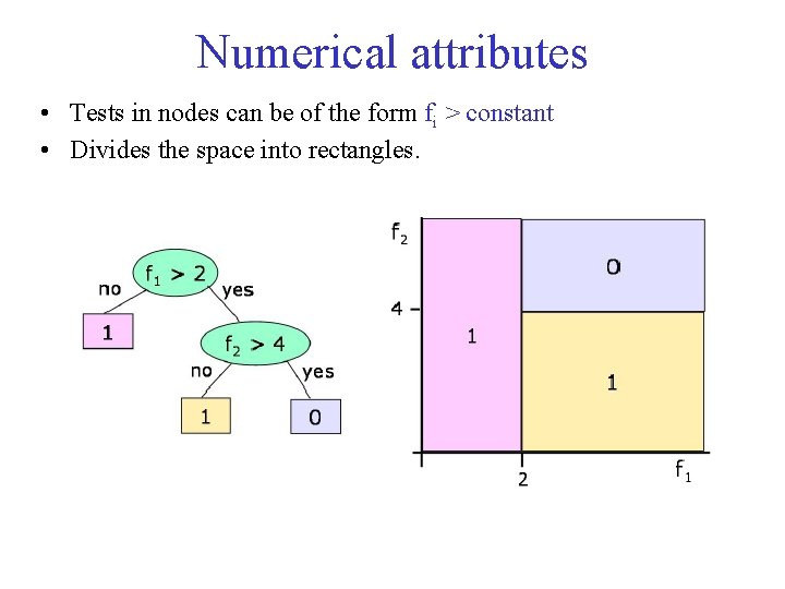
Numerical attributes • Tests in nodes can be of the form fi > constant • Divides the space into rectangles.

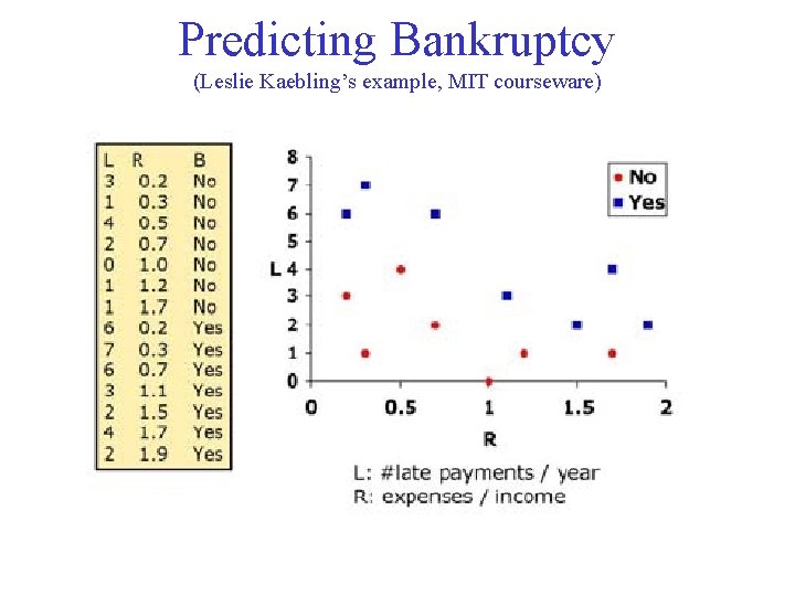
Predicting Bankruptcy (Leslie Kaebling’s example, MIT courseware)

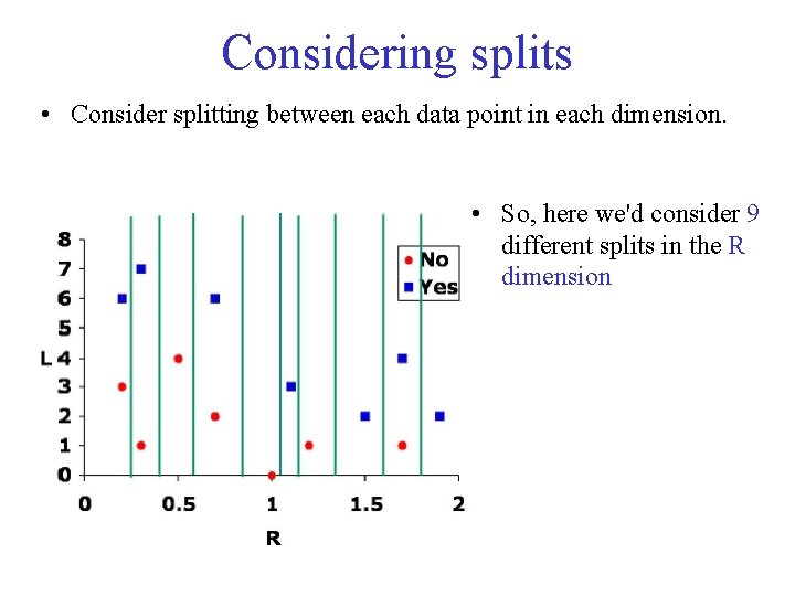
Considering splits • Consider splitting between each data point in each dimension. • So, here we'd consider 9 different splits in the R dimension

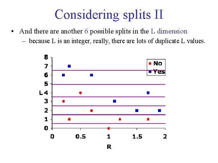
Considering splits II • And there another 6 possible splits in the L dimension – because L is an integer, really, there are lots of duplicate L values.

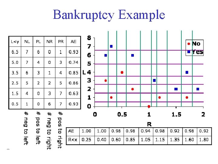
Bankruptcy Example

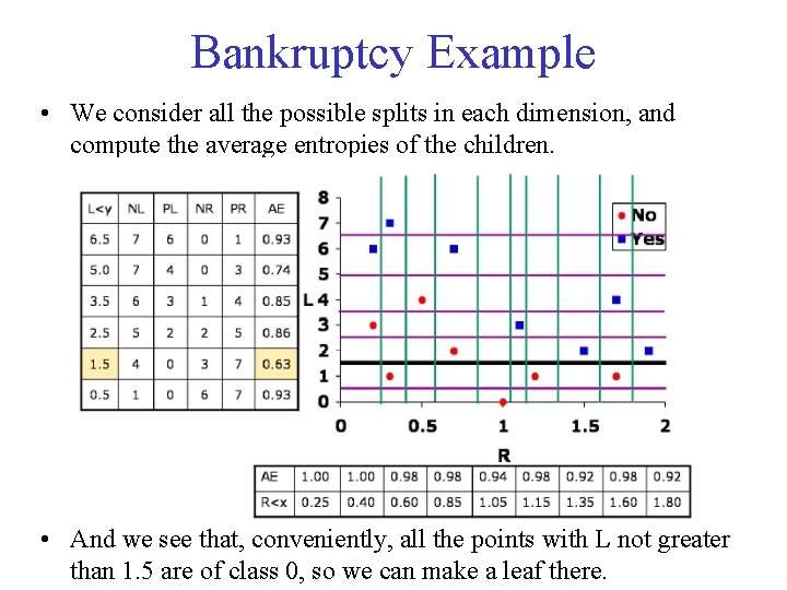
Bankruptcy Example • We consider all the possible splits in each dimension, and compute the average entropies of the children. • And we see that, conveniently, all the points with L not greater than 1. 5 are of class 0, so we can make a leaf there.

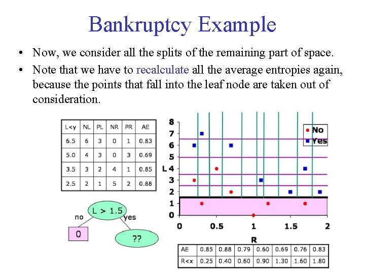
Bankruptcy Example • Now, we consider all the splits of the remaining part of space. • Note that we have to recalculate all the average entropies again, because the points that fall into the leaf node are taken out of consideration.

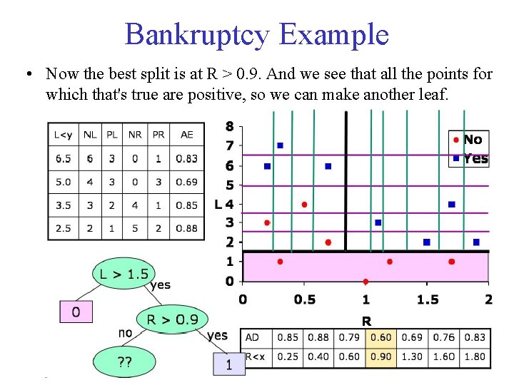
Bankruptcy Example • Now the best split is at R > 0. 9. And we see that all the points for which that's true are positive, so we can make another leaf.

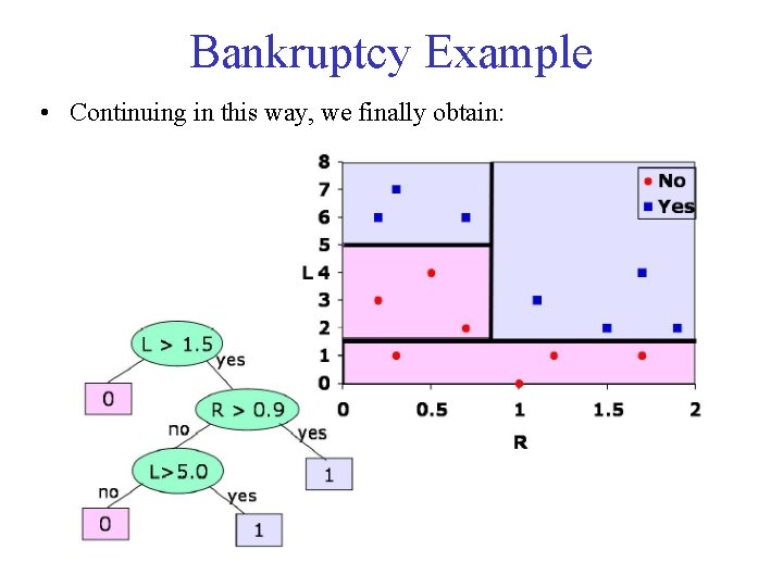
Bankruptcy Example • Continuing in this way, we finally obtain:

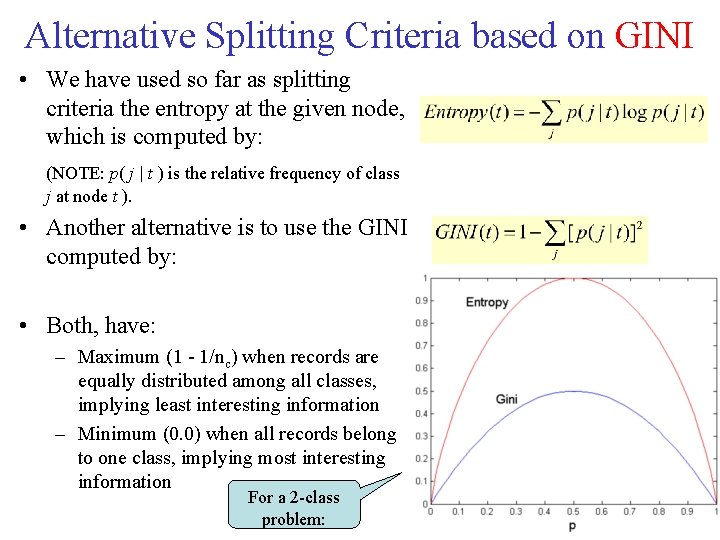
Alternative Splitting Criteria based on GINI • We have used so far as splitting criteria the entropy at the given node, which is computed by: (NOTE: p( j | t ) is the relative frequency of class j at node t ). • Another alternative is to use the GINI computed by: • Both, have: – Maximum (1 - 1/nc) when records are equally distributed among all classes, implying least interesting information – Minimum (0. 0) when all records belong to one class, implying most interesting information For a 2 -class problem:

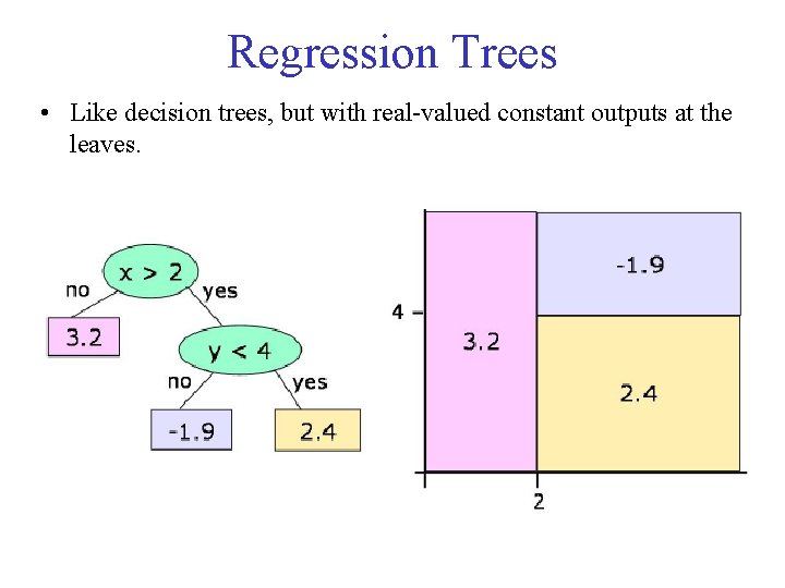
Regression Trees • Like decision trees, but with real-valued constant outputs at the leaves.

Leaf values • Assume that multiple training points are in the leaf and we have decided, for whatever reason, to stop splitting. – In the boolean case, we use the majority output value as the value for the leaf. – In the numeric case, we'll use the average output value. • So, if we're going to use the average value at a leaf as its output, we'd like to split up the data so that the leaf averages are not too far away from the actual items in the leaf. • Statistics has a good measure of how spread out a set of numbers is – (and, therefore, how different the individuals are from the average); – it's called the variance of a set.

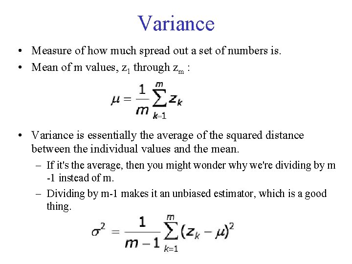
Variance • Measure of how much spread out a set of numbers is. • Mean of m values, z 1 through zm : • Variance is essentially the average of the squared distance between the individual values and the mean. – If it's the average, then you might wonder why we're dividing by m -1 instead of m. – Dividing by m-1 makes it an unbiased estimator, which is a good thing.

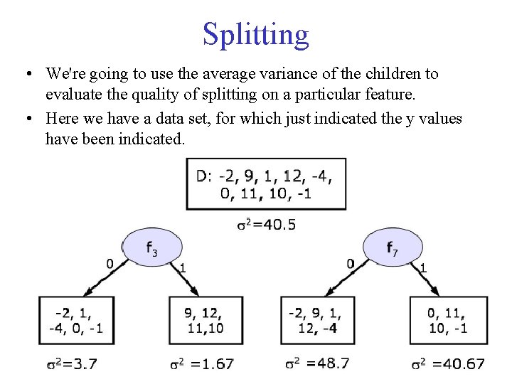
Splitting • We're going to use the average variance of the children to evaluate the quality of splitting on a particular feature. • Here we have a data set, for which just indicated the y values have been indicated.

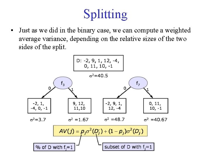
Splitting • Just as we did in the binary case, we can compute a weighted average variance, depending on the relative sizes of the two sides of the split.

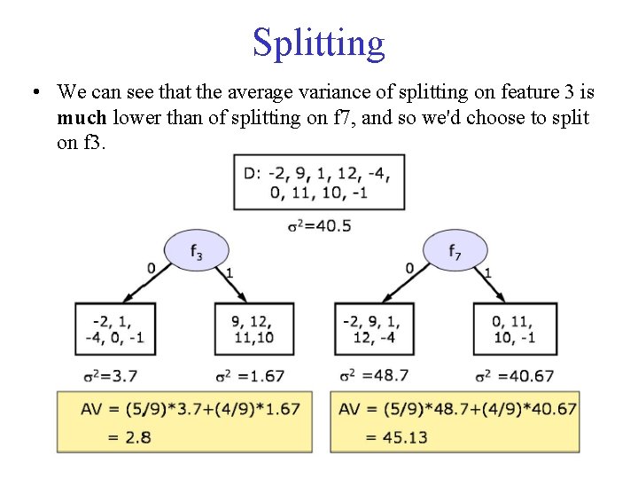
Splitting • We can see that the average variance of splitting on feature 3 is much lower than of splitting on f 7, and so we'd choose to split on f 3.

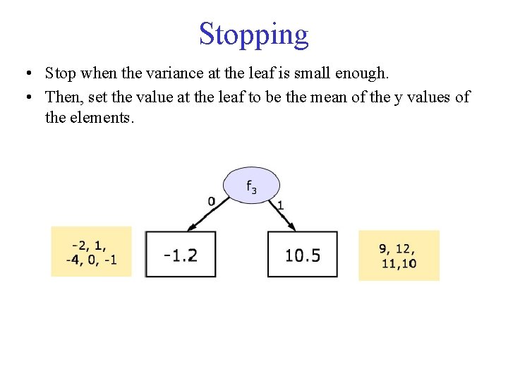
Stopping • Stop when the variance at the leaf is small enough. • Then, set the value at the leaf to be the mean of the y values of the elements.