Decision Tree Shilpa Sonawani Binary decision trees A

Decision Tree Shilpa Sonawani

Binary decision trees • A binary decision tree is a structure based on a sequential decision process • Starting from the root, a feature is evaluated and one of the two branches is selected. • This procedure is repeated until a final leaf is reached, which normally represents the classification target we’re looking for. • decision trees can work efficiently with unnormalized datasets because their internal structure is not influenced by the values assumed by each feature.

Algorithm for Decision Tree Induction • Basic algorithm (a greedy algorithm) – Tree is constructed in a top-down recursive divide-and-conquer manner – At start, all the training examples are at the root – Attributes are categorical (if continuous-valued, they are discretized in advance) – Examples are partitioned recursively based on selected attributes – Test attributes are selected on the basis of a heuristic or statistical measure (e. g. , information gain) • Conditions for stopping partitioning – All samples for a given node belong to the same class – There are no remaining attributes for further partitioning – majority voting is employed for classifying the leaf – There are no samples left 3

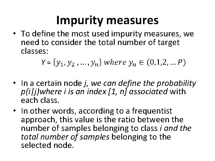
Impurity measures • To define the most used impurity measures, we need to consider the total number of target classes: • In a certain node j, we can define the probability p(i|j)where i is an index [1, n] associated with each class. • In other words, according to a frequentist approach, this value is the ratio between the number of samples belonging to class i and the total number of samples belonging to the selected node.

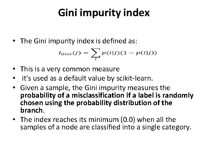
Gini impurity index • The Gini impurity index is defined as: • This is a very common measure • it's used as a default value by scikit-learn. • Given a sample, the Gini impurity measures the probability of a misclassification if a label is randomly chosen using the probability distribution of the branch. • The index reaches its minimum (0. 0) when all the samples of a node are classified into a single category.

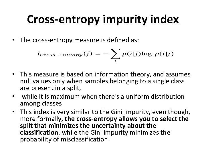
Cross-entropy impurity index • The cross-entropy measure is defined as: • This measure is based on information theory, and assumes null values only when samples belonging to a single class are present in a split, • while it is maximum when there's a uniform distribution among classes • This index is very similar to the Gini impurity, even though, more formally, the cross-entropy allows you to select the split that minimizes the uncertainty about the classification, while the Gini impurity minimizes the probability of misclassification.

• When growing a tree, we start by selecting the split that provides the highest information gain and proceed until one of the following conditions is verified: • All nodes are pure • The information gain is null • The maximum depth has been reached

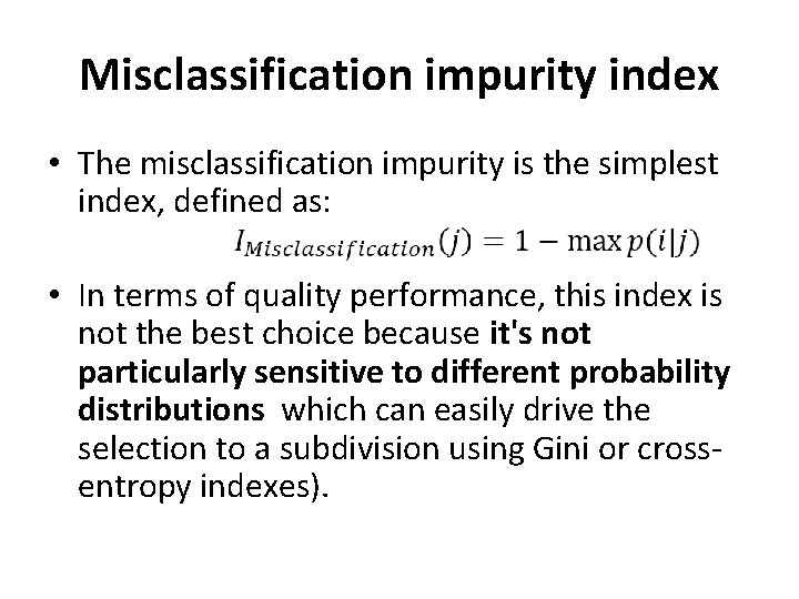
Misclassification impurity index • The misclassification impurity is the simplest index, defined as: • In terms of quality performance, this index is not the best choice because it's not particularly sensitive to different probability distributions which can easily drive the selection to a subdivision using Gini or crossentropy indexes).

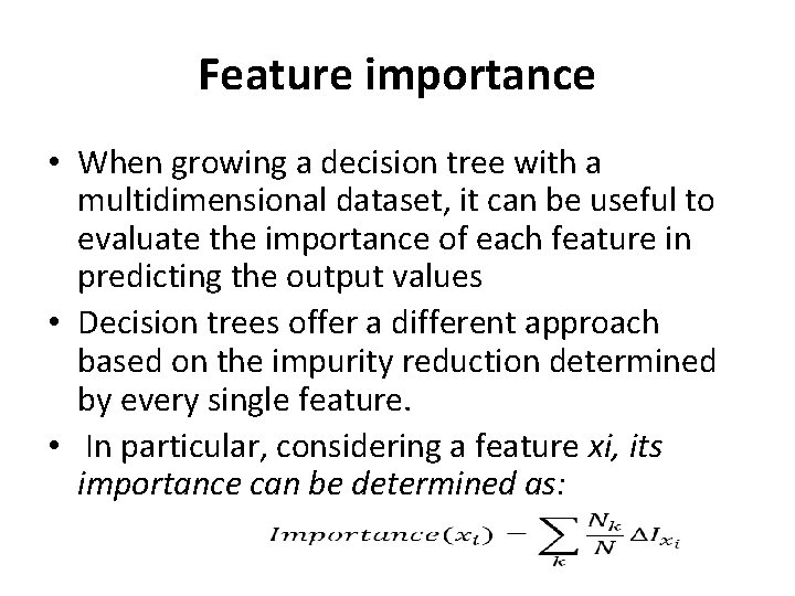
Feature importance • When growing a decision tree with a multidimensional dataset, it can be useful to evaluate the importance of each feature in predicting the output values • Decision trees offer a different approach based on the impurity reduction determined by every single feature. • In particular, considering a feature xi, its importance can be determined as:

• The sum is extended to all nodes where xi is used, and Nk is the number of samples reaching the node k. • Therefore, the importance is a weighted sum of all impurity reductions computed considering only the nodes where the feature is used to split them. • If the Gini impurity index is adopted, this measure is also called Gini importance.

Decision tree classification with scikitlearn • from sklearn. datasets import make_classification • >>> nb_samples = 500 • >>> X, Y = make_classification(n_samples=nb_samples, n_features=3, • n_informative=3, n_redundant=0, n_classes=3, n_clusters_per_class=1)

classification with default Gini impurity • from sklearn. tree import Decision. Tree. Classifier • from sklearn. model_selection import cross_val_score • >>> dt = Decision. Tree. Classifier() • >>> print(cross_val_score(dt, X, Y, scoring='accuracy', cv=10). mean()) • 0. 970

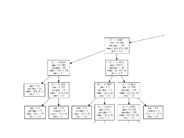
• To export a trained tree, it is necessary to use the built-in function export_graphviz(): • from sklearn. tree import export_graphviz • >>> dt. fit(X, Y) • >>> with open('dt. dot', 'w') as df: • df = export_graphviz(dt, out_file=df, • feature_names=['A', 'B', 'C'], • class_names=['C 1', 'C 2', 'C 3']) • In this case, we have used A, B, and C as feature names and C 1, C 2, and C 3 as class names

• Once the file has been created, it's possible converting to PDF using the command-line tool: • >>> <Graphviz Home>bindot -Tpdf dt. dot -o dt. pdf

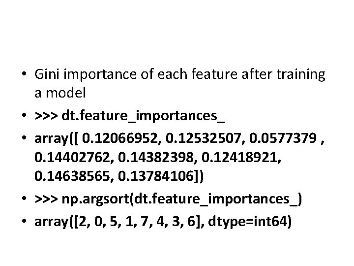
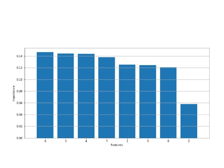
• Gini importance of each feature after training a model • >>> dt. feature_importances_ • array([ 0. 12066952, 0. 12532507, 0. 0577379 , 0. 14402762, 0. 14382398, 0. 12418921, 0. 14638565, 0. 13784106]) • >>> np. argsort(dt. feature_importances_) • array([2, 0, 5, 1, 7, 4, 3, 6], dtype=int 64)

• In terms of efficiency, a tree can also be pruned using the • max_depth parameter: it's not always so simple to understand which value is the best (grid search can help in this task). • On the other hand, it's easier to decide what the maximum number of features to consider at each split should be using max_features • Another parameter useful for controlling both performance and efficiency is min_samples_split which specifies the minimum number of samples to consider for a split

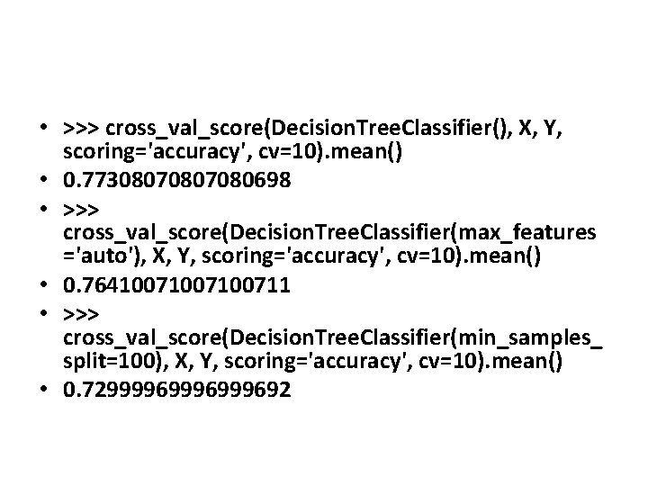
• >>> cross_val_score(Decision. Tree. Classifier(), X, Y, scoring='accuracy', cv=10). mean() • 0. 7730807080698 • >>> cross_val_score(Decision. Tree. Classifier(max_features ='auto'), X, Y, scoring='accuracy', cv=10). mean() • 0. 7641007100711 • >>> cross_val_score(Decision. Tree. Classifier(min_samples_ split=100), X, Y, scoring='accuracy', cv=10). mean() • 0. 7299996999692

• As already explained, finding the best parameters is generally a difficult task, and the best way to carry it out is to perform a grid search while including all the values that could affect the accuracy.

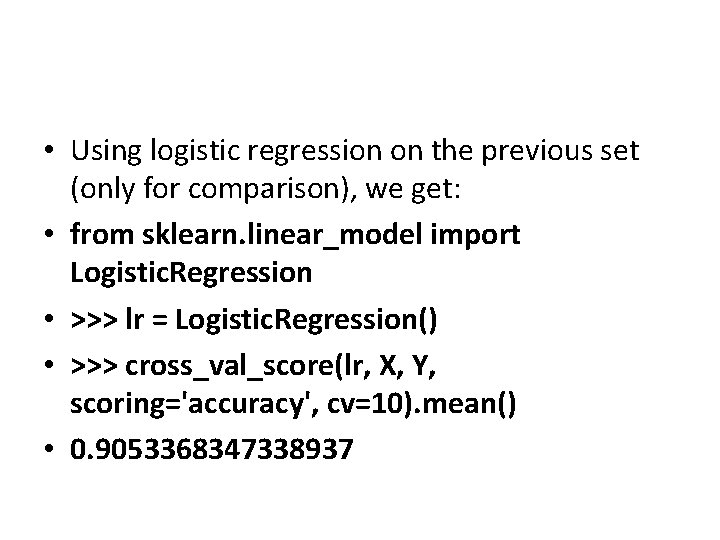
• Using logistic regression on the previous set (only for comparison), we get: • from sklearn. linear_model import Logistic. Regression • >>> lr = Logistic. Regression() • >>> cross_val_score(lr, X, Y, scoring='accuracy', cv=10). mean() • 0. 9053368347338937

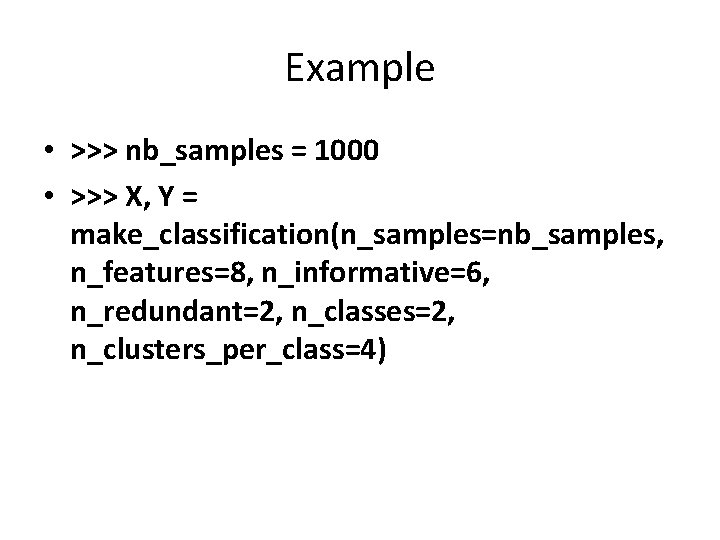
Example • >>> nb_samples = 1000 • >>> X, Y = make_classification(n_samples=nb_samples, n_features=8, n_informative=6, n_redundant=2, n_classes=2, n_clusters_per_class=4)

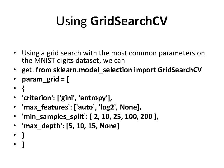
Using Grid. Search. CV • Using a grid search with the most common parameters on the MNIST digits dataset, we can • get: from sklearn. model_selection import Grid. Search. CV • param_grid = [ • { • 'criterion': ['gini', 'entropy'], • 'max_features': ['auto', 'log 2', None], • 'min_samples_split': [ 2, 10, 25, 100, 200 ], • 'max_depth': [5, 10, 15, None] • } • ]

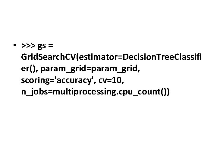
• >>> gs = Grid. Search. CV(estimator=Decision. Tree. Classifi er(), param_grid=param_grid, scoring='accuracy', cv=10, n_jobs=multiprocessing. cpu_count())

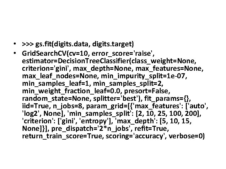
• >>> gs. fit(digits. data, digits. target) • Grid. Search. CV(cv=10, error_score='raise', estimator=Decision. Tree. Classifier(class_weight=None, criterion='gini', max_depth=None, max_features=None, max_leaf_nodes=None, min_impurity_split=1 e-07, min_samples_leaf=1, min_samples_split=2, min_weight_fraction_leaf=0. 0, presort=False, random_state=None, splitter='best'), fit_params={}, iid=True, n_jobs=8, param_grid=[{'max_features': ['auto', 'log 2', None], 'min_samples_split': [2, 10, 25, 100, 200], 'criterion': ['gini', 'entropy'], 'max_depth': [5, 10, 15, None]}], pre_dispatch='2*n_jobs', refit=True, return_train_score=True, scoring='accuracy', verbose=0)

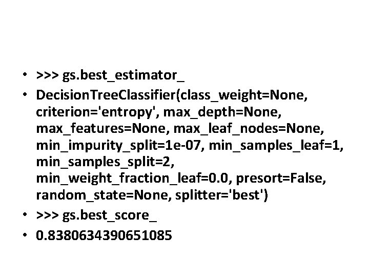
• >>> gs. best_estimator_ • Decision. Tree. Classifier(class_weight=None, criterion='entropy', max_depth=None, max_features=None, max_leaf_nodes=None, min_impurity_split=1 e-07, min_samples_leaf=1, min_samples_split=2, min_weight_fraction_leaf=0. 0, presort=False, random_state=None, splitter='best') • >>> gs. best_score_ • 0. 8380634390651085

Ensemble methods • Ensemble methods are a powerful alternative to complex algorithms because they try to exploit the statistical concept of majority vote • Many weak learners can be trained to capture different elements and make their own predictions, which are not globally optimal • But using a sufficient number of elements, it's statistically probable that a majority will evaluate correctly. • Random forests of decision trees can be used • Boosting methods can be used that are slightly different algorithms that can optimize the learning process by focusing on misclassified samples or by continuously minimizing a target loss • function.

Ensemble learning • Weak learners can be trained in parallel or sequentially (with slight modifications on the parameters) and used as an ensemble based on a majority vote or the averaging of results. • These methods can be classified into two main categories: • Bagged (or Bootstrap) trees: • In this case, the ensemble is built completely. The training process is based on a random selection of the splits and the predictions are based on a majority vote. Random forests are an example of bagged tree ensembles. • Boosted trees: • The ensemble is built sequentially, focusing on the samples that have been previously misclassified. Examples of boosted trees are Ada. Boost and gradient tree boosting.

Random forests • A random forest is a set of decision trees built on random samples with a different policy for splitting a node • Instead of looking for the best choice, in such a model, a random subset of features (for each tree) is used, trying to find the threshold that best separates the data. • As a result, there will be many trees trained in a weaker way and each of them will produce a different prediction.

• There are two ways to interpret these results; the more common approach is based on a majority vote (the most voted class will be considered correct). • However, scikit-learn implements an algorithm based on averaging the results, which yields very accurate predictions.

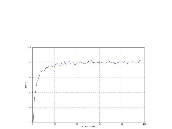
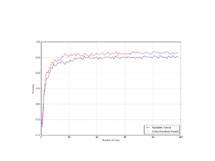
• As an example, let's consider the MNIST dataset with random forests made of a different number of trees: • from sklearn. ensemble import Random. Forest. Classifier • >>> nb_classifications = 100 • >>> accuracy = [] • >>> for i in range(1, nb_classifications): • a= cross_val_score(Random. Forest. Classifier(n_estimators=i), digits. data, digits. target, scoring='accuracy', v=10). mean() • rf_accuracy. append(a)

• the accuracy is low when the number of trees is under a minimum threshold it starts increasing rapidly with fewer than 10 trees

Extra. Trees. Classifier class • Using the Extra. Trees. Classifier class, it's possible to implement a model that randomly computes thresholds and picks the best one. • from sklearn. ensemble import Extra. Trees. Classifier • >>> nb_classifications = 100 • >>> for i in range(1, nb_classifications): • a= cross_val_score(Extra. Trees. Classifier(n_estimators=i), digits. data, digits. target, scoring='accuracy', cv=10). mean() • et_accuracy. append(a)

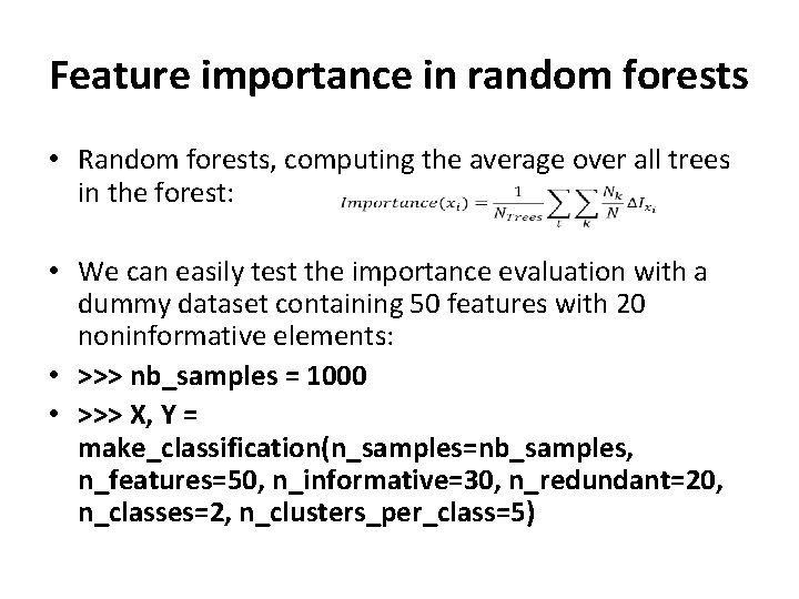
Feature importance in random forests • Random forests, computing the average over all trees in the forest: • We can easily test the importance evaluation with a dummy dataset containing 50 features with 20 noninformative elements: • >>> nb_samples = 1000 • >>> X, Y = make_classification(n_samples=nb_samples, n_features=50, n_informative=30, n_redundant=20, n_classes=2, n_clusters_per_class=5)

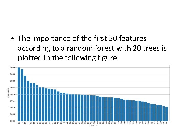
• The importance of the first 50 features according to a random forest with 20 trees is plotted in the following figure:

• Using decision trees or random forests, it's possible to assess the "real" importance of all features and exclude all the elements under a fixed threshold. • In this way, a complex decision process can be simplified and, at the same time, be partially denoised.

Ada. Boost • Ada. Boost (short for Adaptive Boosting) • The basic structure behind this can be a decision tree • But the dataset used for training is continuously adapted to force the model to focus on those samples that are misclassified. • Classifiers are added sequentially, so a new one boosts the previous one by improving the performance in those areas where it was not as accurate as expected. • At each iteration, a weight factor is applied to each sample so as to increase the importance of the samples that are wrongly predicted and decrease the importance of others. • In other words, the model is repeatedly boosted, starting as a very weak learner until the maximum n_estimators number is reached. • The predictions, in this case, are always obtained by majority vote.

• In the scikit-learn implementation, there's also a parameter called learning_rate that weighs the effect of each classifier. • The default value is 1. 0, so all estimators are considered to have the same importance

• However, as we can see with the MNIST dataset, it's useful to decrease this value so that each contribution is weakened: • from sklearn. ensemble import Ada. Boost. Classifier • >>> accuracy = [] • >>> nb_classifications = 100 • >>> for i in range(1, nb_classifications): • a = cross_val_score(Ada. Boost. Classifier(n_estimators=i, learning_rate=0. 1), digits. data, digits. target, scoring='accuracy', cv=10). mean() • >>> ab_accuracy. append(a)

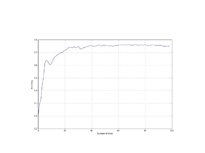
• A grid search on learning_rate could allow you to find the optimal value • A classic random forest, which works with a fixed number of trees since the first iteration, performs better. • This may well be due to the strategy adopted by Ada. Boost; in this set, increasing the weight of the correctly classified samples and decreasing the strength of misclassifications can produce an oscillation in the loss function, with a final result that is not the optimal minimum point

• from sklearn. datasets import load_iris • >>> iris = load_iris() • >>> ada = Ada. Boost. Classifier(n_estimators=100, learning_rate=1. 0) • >>> cross_val_score(ada, iris. data, iris. target, scoring='accuracy', • cv=10). mean() • 0. 9466666666

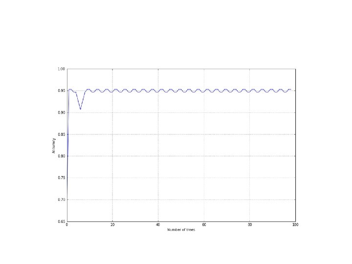
• Boosting process can be stopped after a few iterations • After about 10 iterations in the figure, the accuracy becomes stable. • The advantage of using Ada. Boost can be appreciated in terms of resources; it doesn't work with a fully configured set of classifiers and the whole set of samples. • Therefore, it can help save time when training on large datasets.

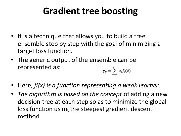
Gradient tree boosting • It is a technique that allows you to build a tree ensemble step by step with the goal of minimizing a target loss function. • The generic output of the ensemble can be represented as: • Here, fi(x) is a function representing a weak learner. • The algorithm is based on the concept of adding a new decision tree at each step so as to minimize the global loss function using the steepest gradient descent method

• scikit-learn implements the Gradient. Boosting. Classifier class, supporting two classification loss functions: • Binomial/multinomial negative log-likelihood (which is the default choice) • Exponential (such as Ada. Boost)

• from sklearn. ensemble import Gradient. Boosting. Classifier • from sklearn. model_selection import cross_val_score • >>> a = [] • >>> max_estimators = 50 • >>> for i in range(1, max_estimators): • >>> score = cross_val_score(Gradient. Boosting. Classifier(n_estimat ors=i, learning_rate=10. 0/float(i)), X, Y, cv=10, scoring='accuracy'). mean() • >>> a. append(score)

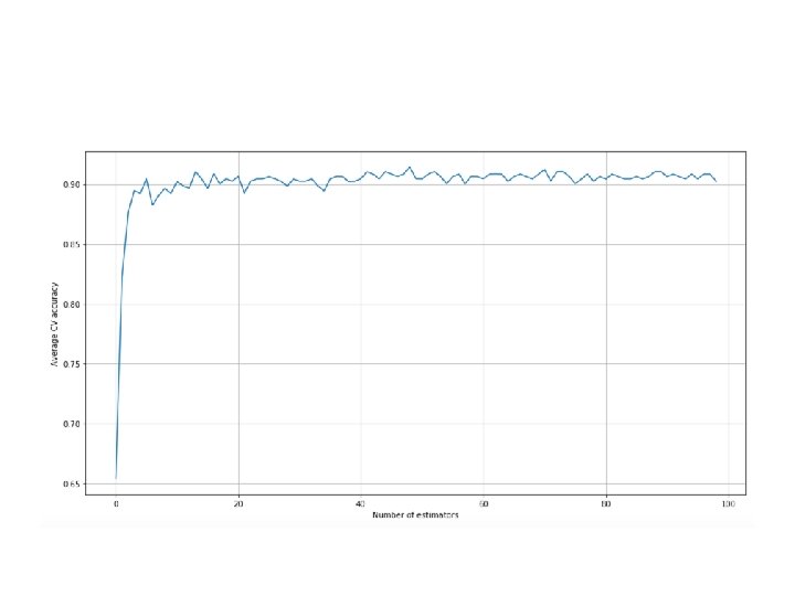
• the cross-validation average accuracy for a number of estimators in the range (1, 50). The loss function is the default one (multinomial negative log-likelihood • While increasing the number of estimators (parameter n_estimators), it's important to decrease the learning rate (parameter learning_rate). The optimal value cannot be easily predicted; therefore, it's often useful to perform a grid search

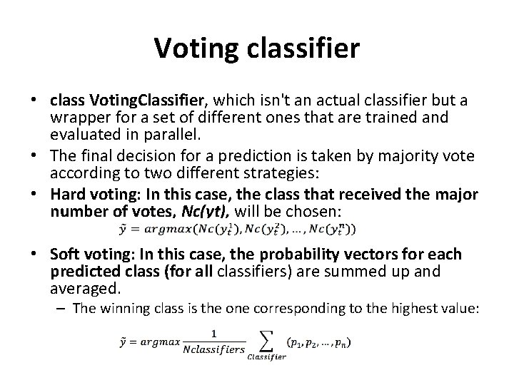
Voting classifier • class Voting. Classifier, which isn't an actual classifier but a wrapper for a set of different ones that are trained and evaluated in parallel. • The final decision for a prediction is taken by majority vote according to two different strategies: • Hard voting: In this case, the class that received the major number of votes, Nc(yt), will be chosen: • Soft voting: In this case, the probability vectors for each predicted class (for all classifiers) are summed up and averaged. – The winning class is the one corresponding to the highest value:

• For our examples, we are going to consider three classifiers: logistic regression, decision tree (with default Gini impurity), and an SVM (with a polynomial kernel and probability=True in order to generate the probability vectors). • When creating an ensemble, it's useful to consider the different features of each involved classifier and avoid "duplicate“ algorithms (for example, a logistic regression and a linear SVM or a perceptron are likely to yield very similar performances). • In many cases, it can be useful to mix nonlinear classifiers with random forests or Ada. Boost classifiers.

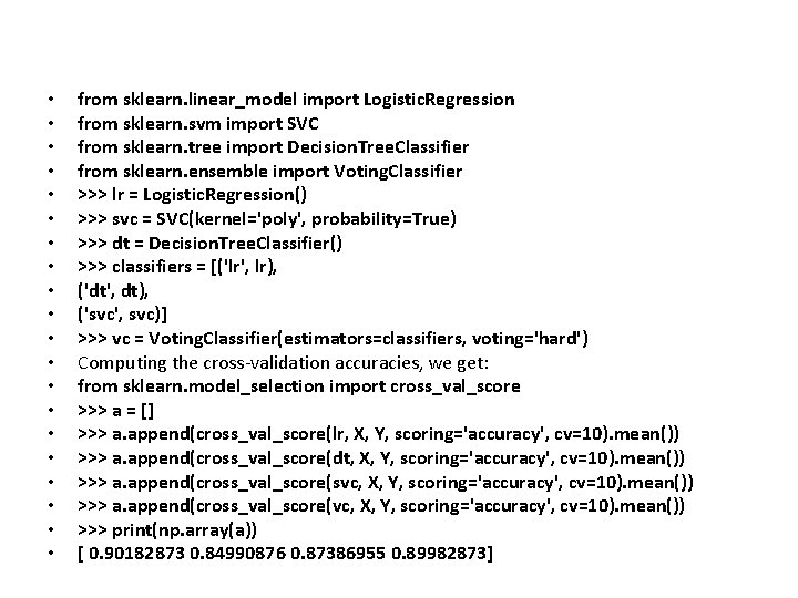
• • • • • from sklearn. linear_model import Logistic. Regression from sklearn. svm import SVC from sklearn. tree import Decision. Tree. Classifier from sklearn. ensemble import Voting. Classifier >>> lr = Logistic. Regression() >>> svc = SVC(kernel='poly', probability=True) >>> dt = Decision. Tree. Classifier() >>> classifiers = [('lr', lr), ('dt', dt), ('svc', svc)] >>> vc = Voting. Classifier(estimators=classifiers, voting='hard') Computing the cross-validation accuracies, we get: from sklearn. model_selection import cross_val_score >>> a = [] >>> a. append(cross_val_score(lr, X, Y, scoring='accuracy', cv=10). mean()) >>> a. append(cross_val_score(dt, X, Y, scoring='accuracy', cv=10). mean()) >>> a. append(cross_val_score(svc, X, Y, scoring='accuracy', cv=10). mean()) >>> a. append(cross_val_score(vc, X, Y, scoring='accuracy', cv=10). mean()) >>> print(np. array(a)) [ 0. 90182873 0. 84990876 0. 87386955 0. 89982873]

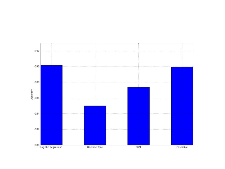
• As expected, the ensemble takes advantage of the different algorithms and yields better performance than any single one.

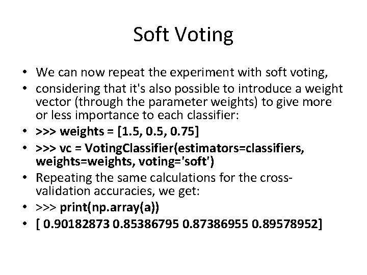
Soft Voting • We can now repeat the experiment with soft voting, • considering that it's also possible to introduce a weight vector (through the parameter weights) to give more or less importance to each classifier: • >>> weights = [1. 5, 0. 75] • >>> vc = Voting. Classifier(estimators=classifiers, weights=weights, voting='soft') • Repeating the same calculations for the crossvalidation accuracies, we get: • >>> print(np. array(a)) • [ 0. 90182873 0. 85386795 0. 87386955 0. 89578952]

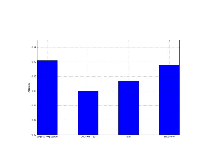
• A voting classifier can be a good choice whenever a single strategy is not able to reach the desired accuracy threshold;