Decision Tree Outline n n Decision tree representation

Decision Tree: Outline n n Decision tree representation ID 3 learning algorithm Entropy, information gain Overfitting Babu Ram Dawadi 1

Defining the Task n Imagine we’ve got a set of data containing several types, or classes. n n E. g. information about customers, and class=whether or not they buy anything. Can we predict, i. e classify, whether a previously unseen customer will buy something? Babu Ram Dawadi 2

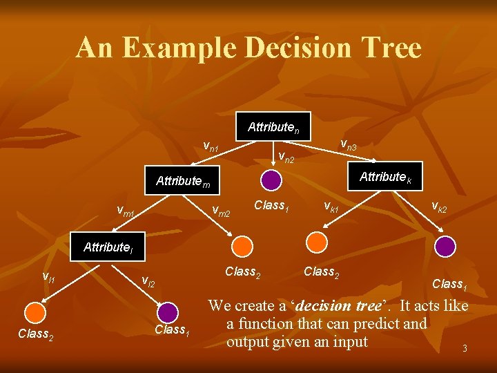
An Example Decision Tree Attributen vn 1 vn 3 vn 2 Attributek Attributem vm 1 vm 2 Class 1 vk 2 Attributel vl 1 Class 2 vl 2 Class 1 Class 2 Class 1 We create a ‘decision tree’. It acts like a function that can predict and output given an input 3

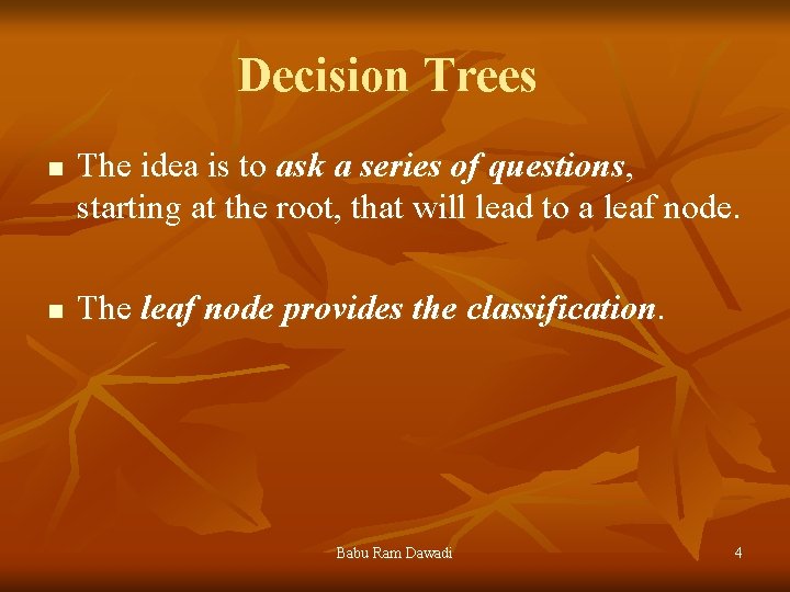
Decision Trees n n The idea is to ask a series of questions, starting at the root, that will lead to a leaf node. The leaf node provides the classification. Babu Ram Dawadi 4

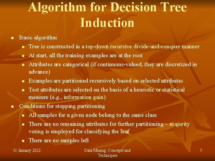
Algorithm for Decision Tree Induction n n Basic algorithm n Tree is constructed in a top-down recursive divide-and-conquer manner n At start, all the training examples are at the root n Attributes are categorical (if continuous-valued, they are discretized in advance) n Examples are partitioned recursively based on selected attributes n Test attributes are selected on the basis of a heuristic or statistical measure (e. g. , information gain) Conditions for stopping partitioning n All samples for a given node belong to the same class n There are no remaining attributes for further partitioning – majority voting is employed for classifying the leaf n There are no samples left 31 January 2022 Data Mining: Concepts and Techniques 5

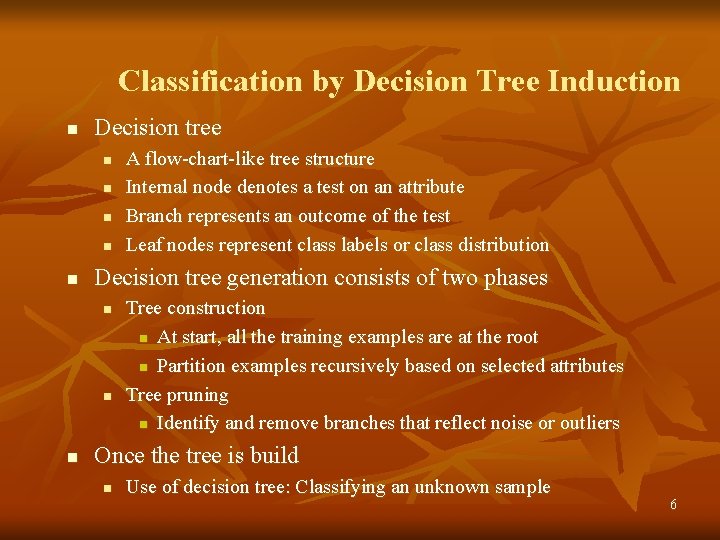
Classification by Decision Tree Induction n Decision tree n n n Decision tree generation consists of two phases n n n A flow-chart-like tree structure Internal node denotes a test on an attribute Branch represents an outcome of the test Leaf nodes represent class labels or class distribution Tree construction n At start, all the training examples are at the root n Partition examples recursively based on selected attributes Tree pruning n Identify and remove branches that reflect noise or outliers Once the tree is build n Use of decision tree: Classifying an unknown sample 6

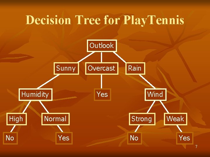
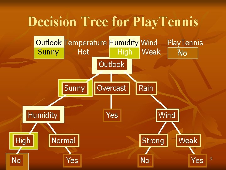
Decision Tree for Play. Tennis Outlook Sunny Humidity High No Overcast Rain Yes Normal Yes Wind Strong No Weak Yes 7

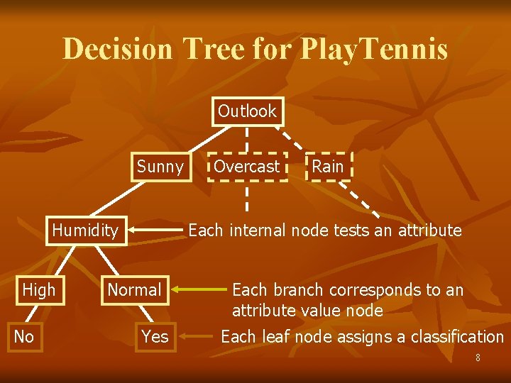
Decision Tree for Play. Tennis Outlook Sunny Humidity High No Overcast Rain Each internal node tests an attribute Normal Yes Each branch corresponds to an attribute value node Each leaf node assigns a classification 8

Decision Tree for Play. Tennis Outlook Temperature Humidity Wind Play. Tennis Sunny Hot High Weak ? No Outlook Sunny Humidity High No Overcast Rain Yes Normal Yes Wind Strong No Weak Yes 9

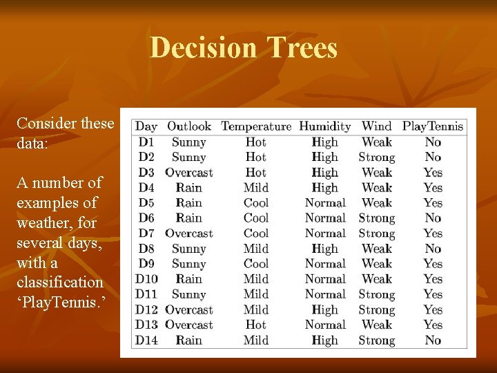
Decision Trees Consider these data: A number of examples of weather, for several days, with a classification ‘Play. Tennis. ’ 10

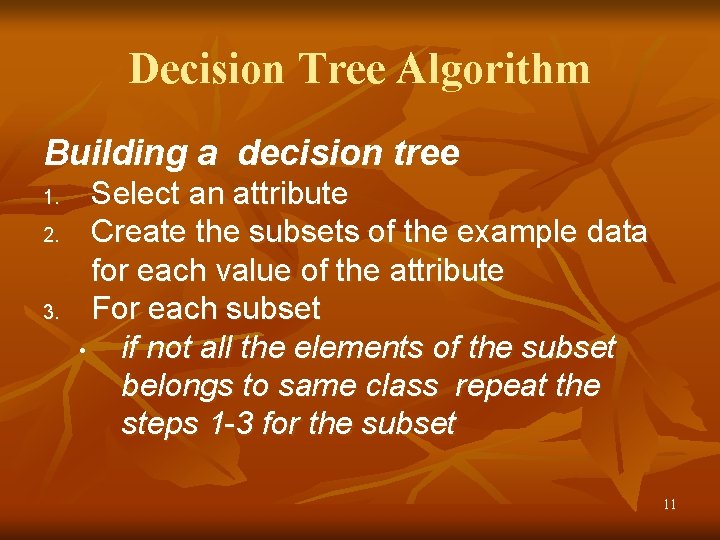
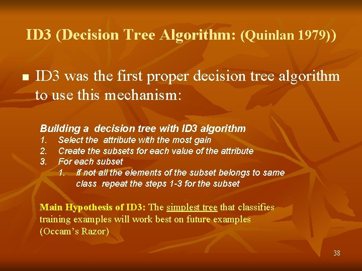
Decision Tree Algorithm Building a decision tree 1. 2. 3. Select an attribute Create the subsets of the example data for each value of the attribute For each subset • if not all the elements of the subset belongs to same class repeat the steps 1 -3 for the subset 11

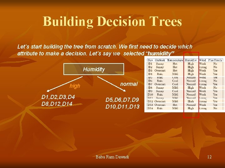
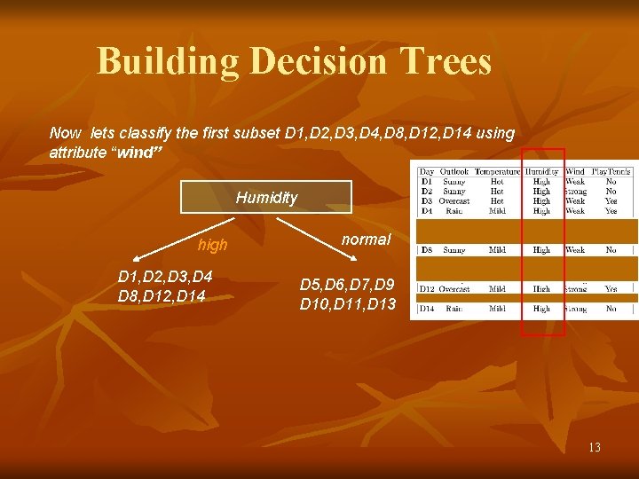
Building Decision Trees Let’s start building the tree from scratch. We first need to decide which attribute to make a decision. Let’s say we selected “humidity” Humidity high D 1, D 2, D 3, D 4 D 8, D 12, D 14 normal D 5, D 6, D 7, D 9 D 10, D 11, D 13 Babu Ram Dawadi 12

Building Decision Trees Now lets classify the first subset D 1, D 2, D 3, D 4, D 8, D 12, D 14 using attribute “wind” Humidity high D 1, D 2, D 3, D 4 D 8, D 12, D 14 normal D 5, D 6, D 7, D 9 D 10, D 11, D 13 13

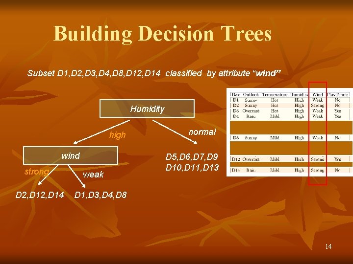
Building Decision Trees Subset D 1, D 2, D 3, D 4, D 8, D 12, D 14 classified by attribute “wind” Humidity high wind strong D 2, D 14 weak normal D 5, D 6, D 7, D 9 D 10, D 11, D 13 D 1, D 3, D 4, D 8 14

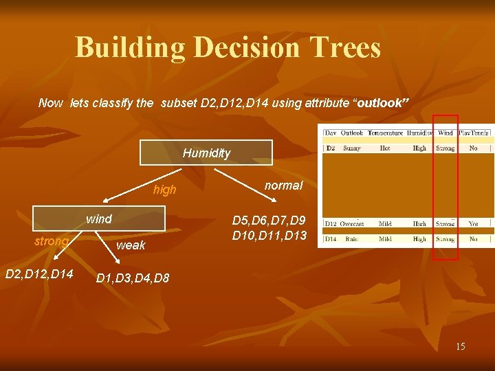
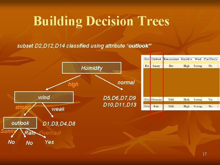
Building Decision Trees Now lets classify the subset D 2, D 14 using attribute “outlook” Humidity high wind strong D 2, D 14 weak normal D 5, D 6, D 7, D 9 D 10, D 11, D 13 D 1, D 3, D 4, D 8 15

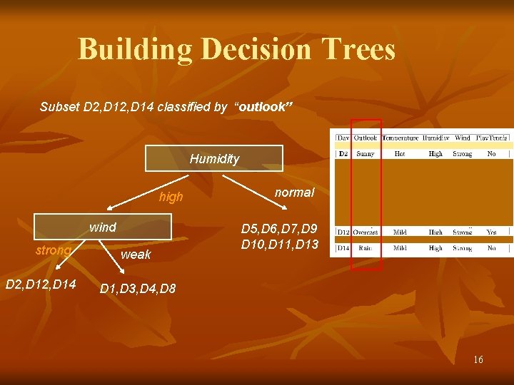
Building Decision Trees Subset D 2, D 14 classified by “outlook” Humidity high wind strong D 2, D 14 weak normal D 5, D 6, D 7, D 9 D 10, D 11, D 13 D 1, D 3, D 4, D 8 16

Building Decision Trees subset D 2, D 14 classified using attribute “outlook” Humidity high wind strong weak normal D 5, D 6, D 7, D 9 D 10, D 11, D 13 outlook D 1, D 3, D 4, D 8 Sunny Rain Overcast No No Yes 17

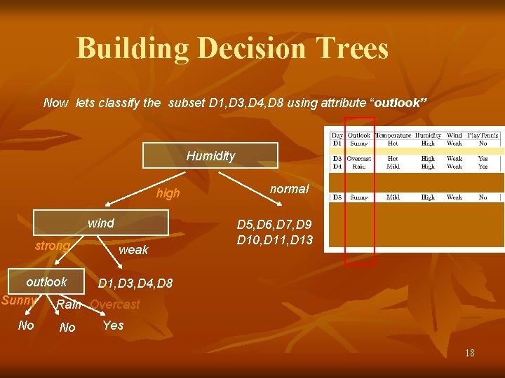
Building Decision Trees Now lets classify the subset D 1, D 3, D 4, D 8 using attribute “outlook” Humidity high wind strong weak normal D 5, D 6, D 7, D 9 D 10, D 11, D 13 outlook D 1, D 3, D 4, D 8 Sunny Rain Overcast No No Yes 18

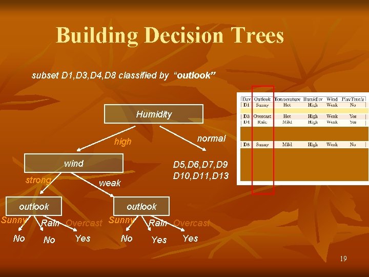
Building Decision Trees subset D 1, D 3, D 4, D 8 classified by “outlook” Humidity normal high wind strong D 5, D 6, D 7, D 9 D 10, D 11, D 13 weak outlook Sunny Rain Overcast No No Yes Yes 19

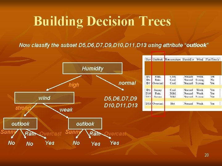
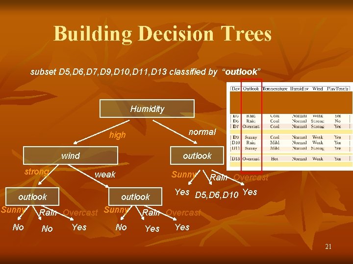
Building Decision Trees Now classify the subset D 5, D 6, D 7, D 9, D 10, D 11, D 13 using attribute “outlook” Humidity normal high wind strong D 5, D 6, D 7, D 9 D 10, D 11, D 13 weak outlook Sunny Rain Overcast No No Yes Yes 20

Building Decision Trees subset D 5, D 6, D 7, D 9, D 10, D 11, D 13 classified by “outlook” Humidity normal high wind strong outlook weak Sunny Rain Overcast Yes D 5, D 6, D 10 Yes outlook Sunny Rain Overcast No No Yes Yes 21

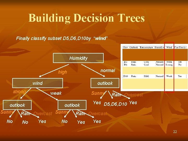
Building Decision Trees Finally classify subset D 5, D 6, D 10 by “wind” Humidity normal high wind strong outlook weak Sunny Rain Overcast Yes D 5, D 6, D 10 Yes outlook Sunny Rain Overcast No No Yes Yes 22

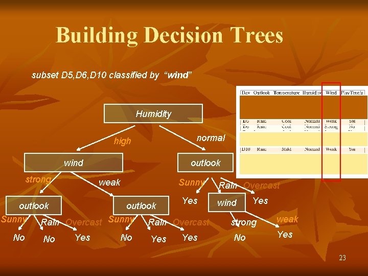
Building Decision Trees subset D 5, D 6, D 10 classified by “wind” Humidity high wind strong normal outlook weak Sunny Rain Overcast Yes wind outlook Sunny Rain Overcast weak strong Yes No No Yes 23

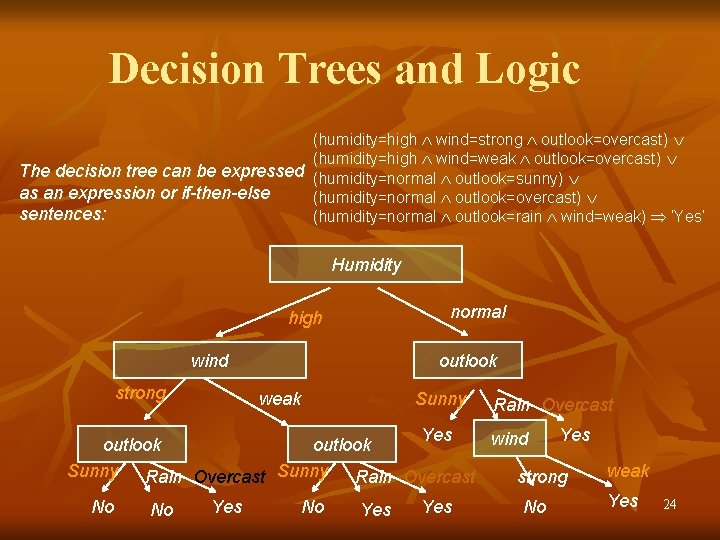
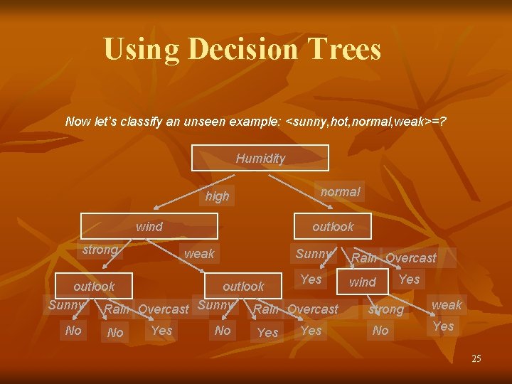
Decision Trees and Logic (humidity=high wind=strong outlook=overcast) (humidity=high wind=weak outlook=overcast) The decision tree can be expressed (humidity=normal outlook=sunny) as an expression or if-then-else (humidity=normal outlook=overcast) sentences: (humidity=normal outlook=rain wind=weak) ‘Yes’ Humidity high wind strong normal outlook weak Sunny Rain Overcast Yes wind outlook Sunny Rain Overcast weak strong Yes No No Yes 24

Using Decision Trees Now let’s classify an unseen example: <sunny, hot, normal, weak>=? Humidity high wind strong normal outlook weak Sunny Rain Overcast Yes wind outlook Sunny Rain Overcast weak strong Yes No No Yes 25

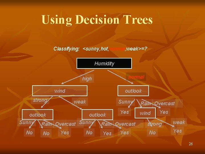
Using Decision Trees Classifying: <sunny, hot, normal, weak>=? Humidity high wind strong normal outlook weak Sunny Rain Overcast Yes wind outlook Sunny Rain Overcast weak strong Yes No No Yes 26

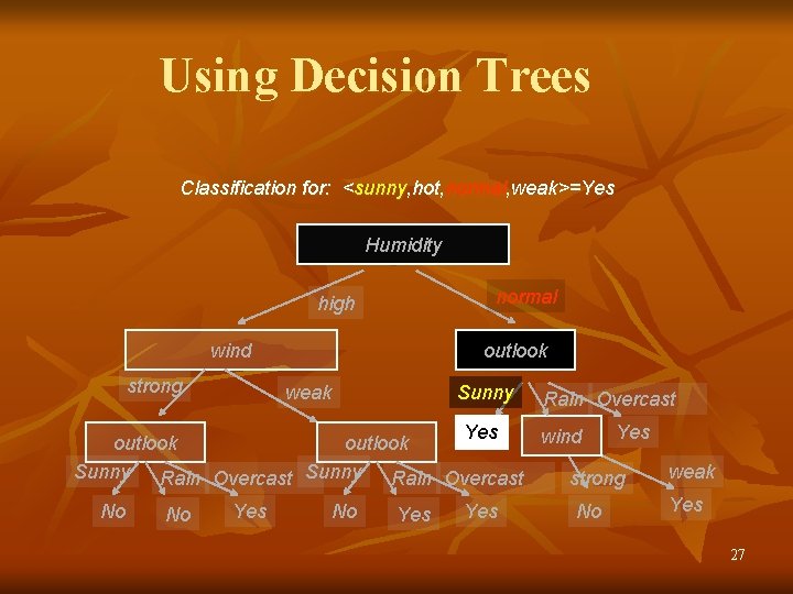
Using Decision Trees Classification for: <sunny, hot, normal, weak>=Yes Humidity high wind strong normal outlook weak Sunny Rain Overcast Yes wind outlook Sunny Rain Overcast weak strong Yes No No Yes 27

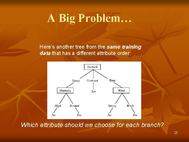
A Big Problem… Here’s another tree from the same training data that has a different attribute order: Which attribute should we choose for each branch? 28

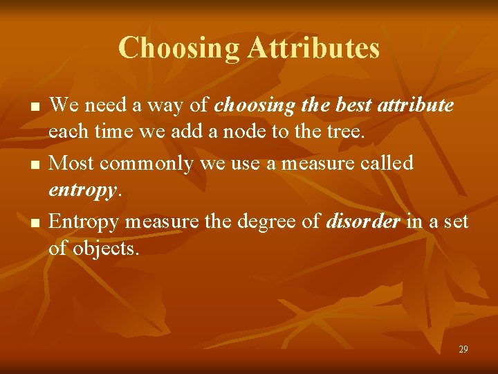
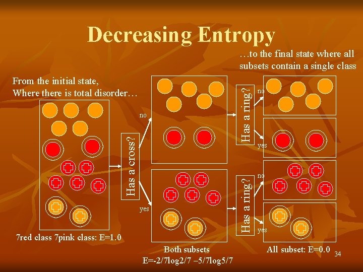
Choosing Attributes n n n We need a way of choosing the best attribute each time we add a node to the tree. Most commonly we use a measure called entropy. Entropy measure the degree of disorder in a set of objects. 29

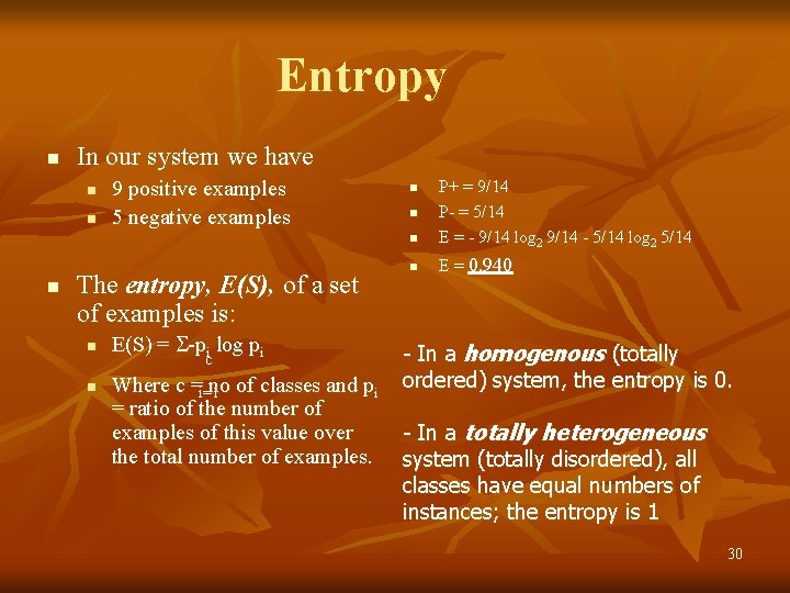
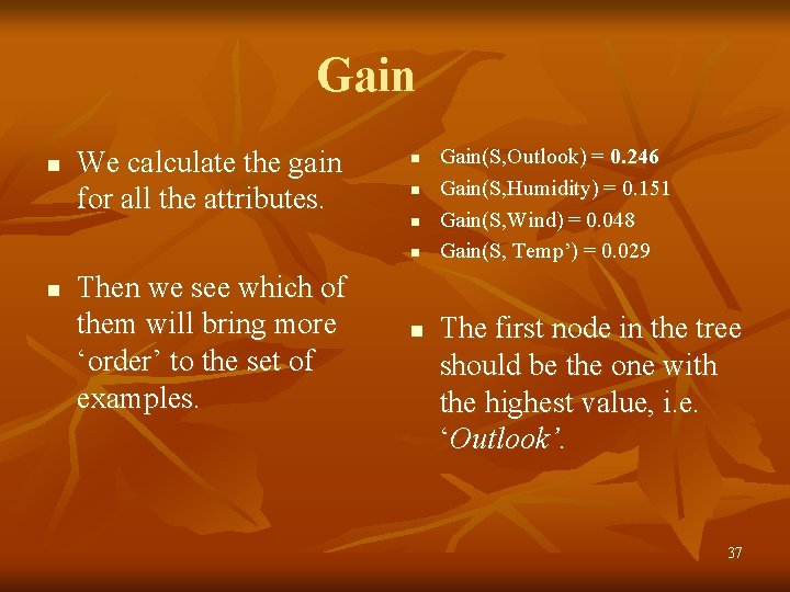
Entropy n In our system we have n n n 9 positive examples 5 negative examples The entropy, E(S), of a set of examples is: n n E(S) = -pi log pi c Where c =i=1 no of classes and pi = ratio of the number of examples of this value over the total number of examples. n P+ = 9/14 P- = 5/14 E = - 9/14 log 2 9/14 - 5/14 log 2 5/14 n E = 0. 940 n n - In a homogenous (totally ordered) system, the entropy is 0. - In a totally heterogeneous system (totally disordered), all classes have equal numbers of instances; the entropy is 1 30

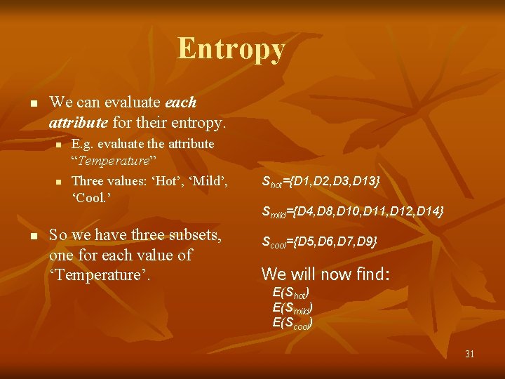
Entropy n We can evaluate each attribute for their entropy. n n n E. g. evaluate the attribute “Temperature” Three values: ‘Hot’, ‘Mild’, ‘Cool. ’ So we have three subsets, one for each value of ‘Temperature’. Shot={D 1, D 2, D 3, D 13} Smild={D 4, D 8, D 10, D 11, D 12, D 14} Scool={D 5, D 6, D 7, D 9} We will now find: E(Shot) E(Smild) E(Scool) 31

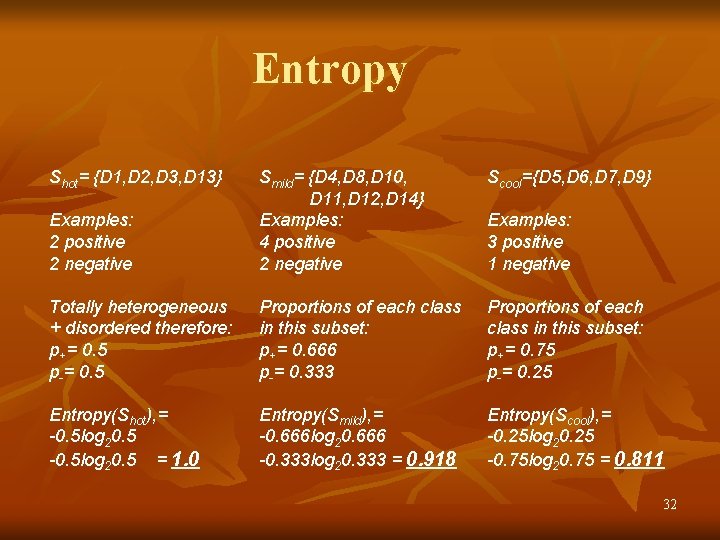
Entropy Shot= {D 1, D 2, D 3, D 13} Scool={D 5, D 6, D 7, D 9} Examples: 2 positive 2 negative Smild= {D 4, D 8, D 10, D 11, D 12, D 14} Examples: 4 positive 2 negative Totally heterogeneous + disordered therefore: p+= 0. 5 p-= 0. 5 Proportions of each class in this subset: p+= 0. 666 p-= 0. 333 Proportions of each class in this subset: p+= 0. 75 p-= 0. 25 Entropy(Shot), = -0. 5 log 20. 5 = 1. 0 Entropy(Smild), = -0. 666 log 20. 666 -0. 333 log 20. 333 = 0. 918 Entropy(Scool), = -0. 25 log 20. 25 -0. 75 log 20. 75 = 0. 811 Examples: 3 positive 1 negative 32

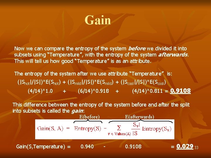
Gain Now we can compare the entropy of the system before we divided it into subsets using “Temperature”, with the entropy of the system afterwards. This will tell us how good “Temperature” is as an attribute. The entropy of the system after we use attribute “Temperature” is: (|Shot|/|S|)*E(Shot) + (|Smild|/|S|)*E(Smild) + (|Scool|/|S|)*E(Scool) (4/14)*1. 0 + (6/14)*0. 918 + (4/14)*0. 811 = 0. 9108 This difference between the entropy of the system before and after the split into subsets is called the gain: E(before) E(afterwards) Gain(S, Temperature) = 0. 940 - 0. 9108 = 0. 029 33

Decreasing Entropy Has a cross? no yes 7 red class 7 pink class: E=1. 0 Both subsets E=-2/7 log 2/7 – 5/7 log 5/7 Has a ring? From the initial state, Where there is total disorder… Has a ring? …to the final state where all subsets contain a single class no yes All subset: E=0. 0 34

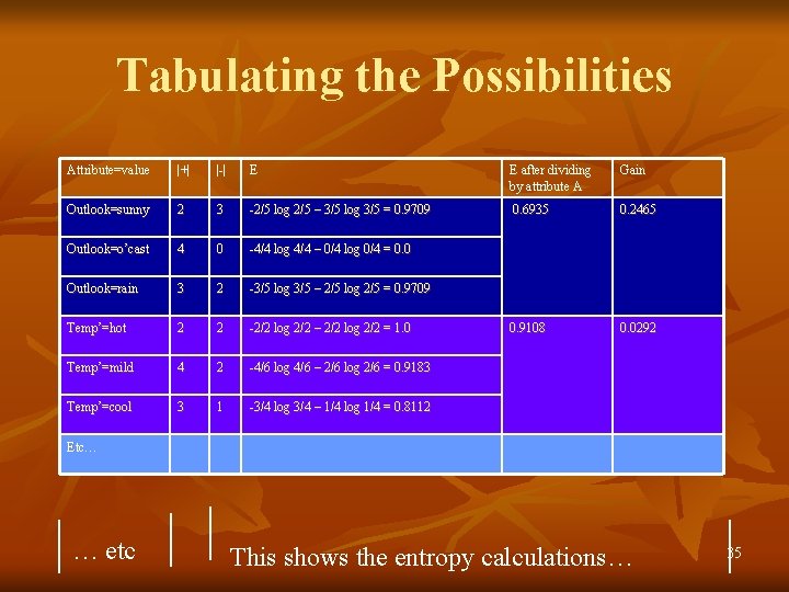
Tabulating the Possibilities Attribute=value |+| |-| E E after dividing by attribute A Gain Outlook=sunny 2 3 -2/5 log 2/5 – 3/5 log 3/5 = 0. 9709 0. 6935 0. 2465 Outlook=o’cast 4 0 -4/4 log 4/4 – 0/4 log 0/4 = 0. 0 Outlook=rain 3 2 -3/5 log 3/5 – 2/5 log 2/5 = 0. 9709 Temp’=hot 2 2 -2/2 log 2/2 – 2/2 log 2/2 = 1. 0 0. 9108 0. 0292 Temp’=mild 4 2 -4/6 log 4/6 – 2/6 log 2/6 = 0. 9183 Temp’=cool 3 1 -3/4 log 3/4 – 1/4 log 1/4 = 0. 8112 Etc… … etc This shows the entropy calculations… 35

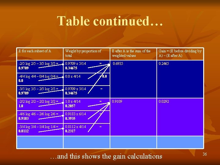
Table continued… E for each subset of A Weight by proportion of total E after A is the sum of the weighted values Gain = (E before dividing by A) – (E after A) -2/5 log 2/5 – 3/5 log 3/5 = 0. 9709 x 5/14 0. 34675 = 0. 6935 0. 2465 -4/4 log 4/4 – 0/4 log 0/4 = 0. 0 x 4/14 = 0. 0 -3/5 log 3/5 – 2/5 log 2/5 = 0. 9709 x 5/14 0. 34675 = -2/2 log 2/2 – 2/2 log 2/2 = 1. 0 x 4/14 0. 2857 = 0. 9109 0. 0292 -4/6 log 4/6 – 2/6 log 2/6 = 0. 9183 x 6/14 0. 3935 = -3/4 log 3/4 – 1/4 log 1/4 = 0. 8112 x 4/14 0. 2317 = …and this shows the gain calculations 36

Gain n We calculate the gain for all the attributes. n n n Then we see which of them will bring more ‘order’ to the set of examples. n Gain(S, Outlook) = 0. 246 Gain(S, Humidity) = 0. 151 Gain(S, Wind) = 0. 048 Gain(S, Temp’) = 0. 029 The first node in the tree should be the one with the highest value, i. e. ‘Outlook’. 37

ID 3 (Decision Tree Algorithm: (Quinlan 1979)) n ID 3 was the first proper decision tree algorithm to use this mechanism: Building a decision tree with ID 3 algorithm 1. 2. 3. Select the attribute with the most gain Create the subsets for each value of the attribute For each subset 1. if not all the elements of the subset belongs to same class repeat the steps 1 -3 for the subset Main Hypothesis of ID 3: The simplest tree that classifies training examples will work best on future examples (Occam’s Razor) 38

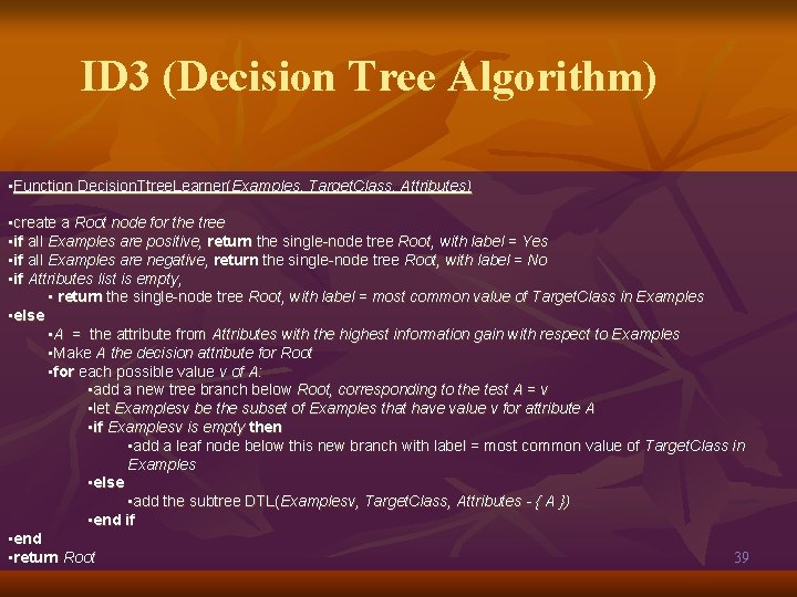
ID 3 (Decision Tree Algorithm) • Function Decision. Ttree. Learner(Examples, Target. Class, Attributes) • create a Root node for the tree • if all Examples are positive, return the single-node tree Root, with label = Yes • if all Examples are negative, return the single-node tree Root, with label = No • if Attributes list is empty, • return the single-node tree Root, with label = most common value of Target. Class in Examples • else • A = the attribute from Attributes with the highest information gain with respect to Examples • Make A the decision attribute for Root • for each possible value v of A: • add a new tree branch below Root, corresponding to the test A = v • let Examplesv be the subset of Examples that have value v for attribute A • if Examplesv is empty then • add a leaf node below this new branch with label = most common value of Target. Class in Examples • else • add the subtree DTL(Examplesv, Target. Class, Attributes - { A }) • end if • end • return Root 39

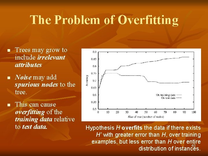
The Problem of Overfitting n n n Trees may grow to include irrelevant attributes Noise may add spurious nodes to the tree. This can cause overfitting of the training data relative to test data. Hypothesis H overfits the data if there exists H’ with greater error than H, over training examples, but less error than H over entire 40 distribution of instances.

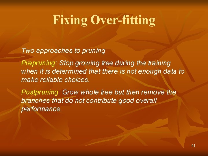
Fixing Over-fitting Two approaches to pruning Prepruning: Stop growing tree during the training when it is determined that there is not enough data to make reliable choices. Postpruning: Grow whole tree but then remove the branches that do not contribute good overall performance. 41

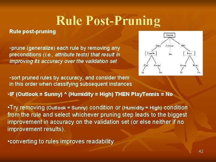
Rule Post-Pruning Rule post-pruning • prune (generalize) each rule by removing any preconditions (i. e. , attribute tests) that result in improving its accuracy over the validation set • sort pruned rules by accuracy, and consider them in this order when classifying subsequent instances • IF (Outlook = Sunny) ^ (Humidity = High) THEN Play. Tennis = No • Try removing (Outlook = Sunny) condition or (Humidity = High) condition from the rule and select whichever pruning step leads to the biggest improvement in accuracy on the validation set (or else neither if no improvement results). • converting to rules improves readability 42

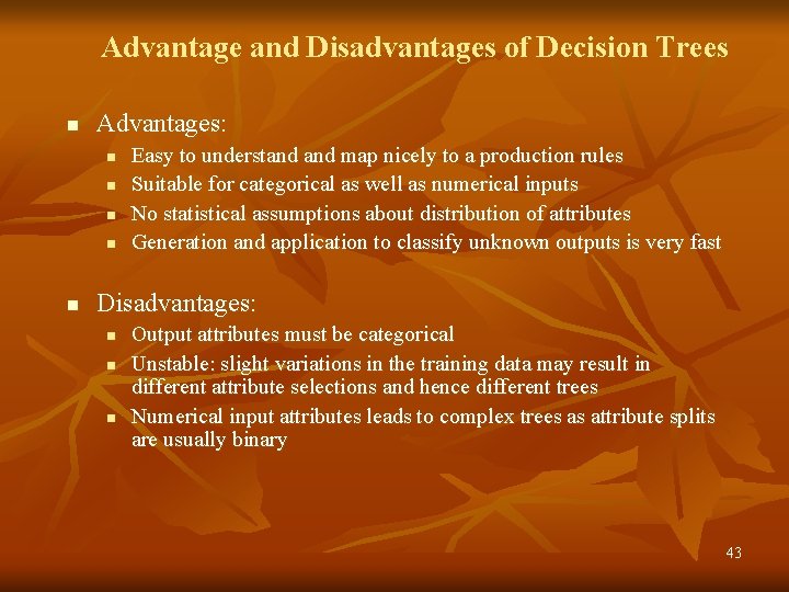
Advantage and Disadvantages of Decision Trees n Advantages: n n n Easy to understand map nicely to a production rules Suitable for categorical as well as numerical inputs No statistical assumptions about distribution of attributes Generation and application to classify unknown outputs is very fast Disadvantages: n n n Output attributes must be categorical Unstable: slight variations in the training data may result in different attribute selections and hence different trees Numerical input attributes leads to complex trees as attribute splits are usually binary 43

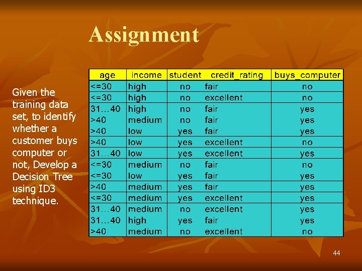
Assignment Given the training data set, to identify whether a customer buys computer or not, Develop a Decision Tree using ID 3 technique. 44

Association Rules n n n Example 1: a female shopper buys a handbag is likely to buy shoes Example 2: when a male customer buys beer, he is likely to buy salted peanuts It is not very difficult to develop algorithms that will find this associations in a large database n The problem is that such an algorithm will also uncover many other associations that are of very little value. 45

Association Rules n n n It is necessary to introduce some measures to distinguish interesting associations from non-interesting ones Look for associations that have a lots of examples in the database: support of an association rule May be that a considerable group of people who read all three magazines but there is a much larger group that buys A & B, but not C; association is very weak here although support might be very high. 46

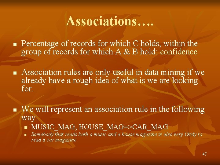
Associations…. n n n Percentage of records for which C holds, within the group of records for which A & B hold: confidence Association rules are only useful in data mining if we already have a rough idea of what is we are looking for. We will represent an association rule in the following way: n n MUSIC_MAG, HOUSE_MAG=>CAR_MAG Somebody that reads both a music and a house magazine is also very likely to read a car magazine 47

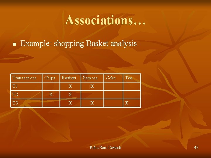
Associations… n Example: shopping Basket analysis Transactions Chips T 1 T 2 T 3 Rasbari X X Samosa Coke Tea X X Babu Ram Dawadi X 48

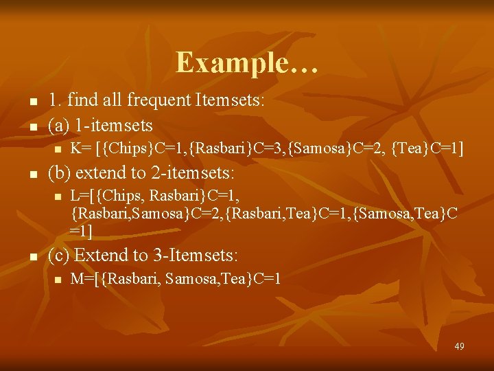
Example… n n 1. find all frequent Itemsets: (a) 1 -itemsets n n (b) extend to 2 -itemsets: n n K= [{Chips}C=1, {Rasbari}C=3, {Samosa}C=2, {Tea}C=1] L=[{Chips, Rasbari}C=1, {Rasbari, Samosa}C=2, {Rasbari, Tea}C=1, {Samosa, Tea}C =1] (c) Extend to 3 -Itemsets: n M=[{Rasbari, Samosa, Tea}C=1 49

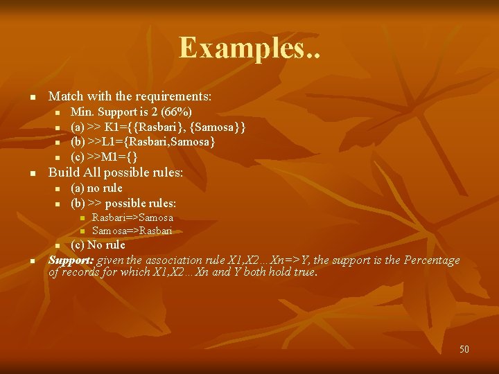
Examples. . n Match with the requirements: n n n Min. Support is 2 (66%) (a) >> K 1={{Rasbari}, {Samosa}} (b) >>L 1={Rasbari, Samosa} (c) >>M 1={} Build All possible rules: n n (a) no rule (b) >> possible rules: n n Rasbari=>Samosa=>Rasbari (c) No rule Support: given the association rule X 1, X 2…Xn=>Y, the support is the Percentage of records for which X 1, X 2…Xn and Y both hold true. n n 50

Example. . n Calculate Confidence for b: n Confidence of [Rasbari=>Samosa] n n Confidence of Samosa=> Rasbari n n {Rasbari, Samosa}C=2/{Rasbari}C=3 =2/3 66% {Rasbari, Samosa}C=2/{Samosa}C=2 =2/2 100% Confidence: Given the association rule X 1, X 2…. Xn=>Y, the confidence is the percentage of records for which Y holds within the group of records for which X 1, X 2…Xn holds true. 51

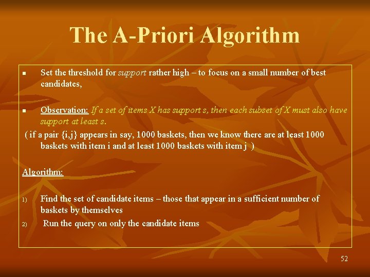
The A-Priori Algorithm n Set the threshold for support rather high – to focus on a small number of best candidates, Observation: If a set of items X has support s, then each subset of X must also have support at least s. ( if a pair {i, j} appears in say, 1000 baskets, then we know there at least 1000 baskets with item i and at least 1000 baskets with item j ) n Algorithm: 1) 2) Find the set of candidate items – those that appear in a sufficient number of baskets by themselves Run the query on only the candidate items 52

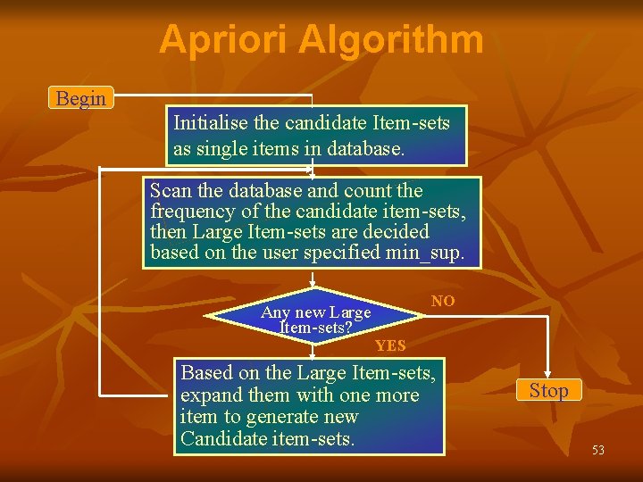
Apriori Algorithm Begin Initialise the candidate Item-sets as single items in database. Scan the database and count the frequency of the candidate item-sets, then Large Item-sets are decided based on the user specified min_sup. Any new Large Item-sets? NO YES Based on the Large Item-sets, expand them with one more item to generate new Candidate item-sets. Stop 53

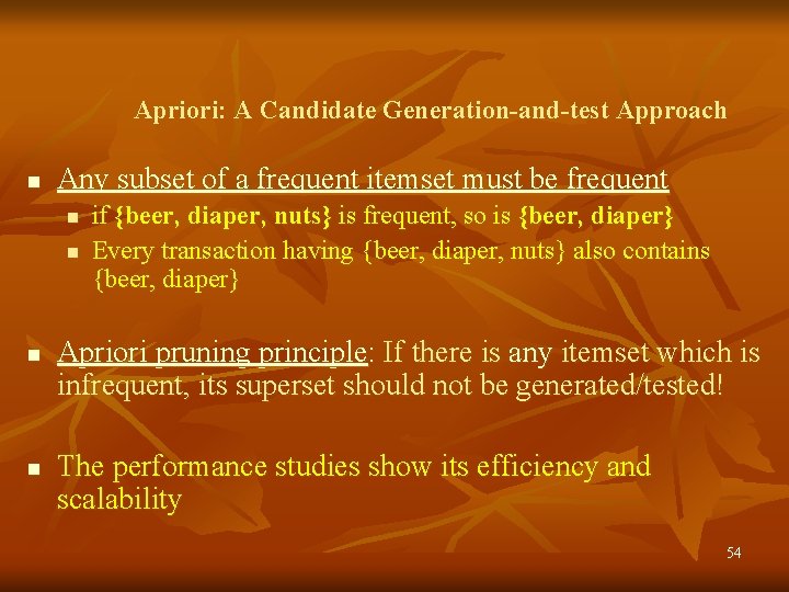
Apriori: A Candidate Generation-and-test Approach n Any subset of a frequent itemset must be frequent n n if {beer, diaper, nuts} is frequent, so is {beer, diaper} Every transaction having {beer, diaper, nuts} also contains {beer, diaper} Apriori pruning principle: If there is any itemset which is infrequent, its superset should not be generated/tested! The performance studies show its efficiency and scalability 54

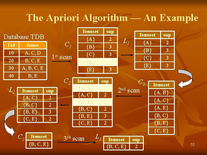
The Apriori Algorithm — An Example Database TDB Tid 10 20 30 40 L 2 C 1 Items A, C, D B, C, E A, B, C, E B, E Itemset {A, C} {B, E} {C, E} C 3 1 st scan C 2 sup 2 2 3 2 Itemset {B, C, E} Itemset {A} {B} {C} {D} {E} Itemset {A, B} {A, C} {A, E} {B, C} {B, E} {C, E} 3 rd scan sup 2 3 3 1 3 sup 1 2 3 2 L 3 L 1 Itemset {A} {B} {C} {E} C 2 2 nd scan Itemset {B, C, E} sup 2 3 3 3 Itemset {A, B} {A, C} {A, E} {B, C} {B, E} {C, E} 55

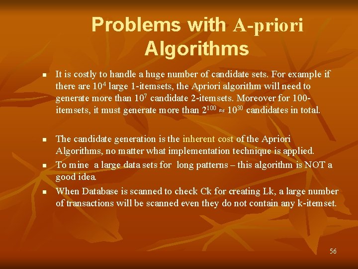
Problems with A-priori Algorithms n n It is costly to handle a huge number of candidate sets. For example if there are 104 large 1 -itemsets, the Apriori algorithm will need to generate more than 107 candidate 2 -itemsets. Moreover for 100 itemsets, it must generate more than 2100 1030 candidates in total. The candidate generation is the inherent cost of the Apriori Algorithms, no matter what implementation technique is applied. To mine a large data sets for long patterns – this algorithm is NOT a good idea. When Database is scanned to check Ck for creating Lk, a large number of transactions will be scanned even they do not contain any k-itemset. 56

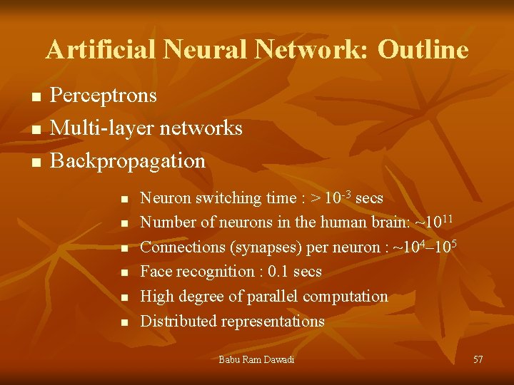
Artificial Neural Network: Outline n n n Perceptrons Multi-layer networks Backpropagation n n n Neuron switching time : > 10 -3 secs Number of neurons in the human brain: ~1011 Connections (synapses) per neuron : ~104– 105 Face recognition : 0. 1 secs High degree of parallel computation Distributed representations Babu Ram Dawadi 57

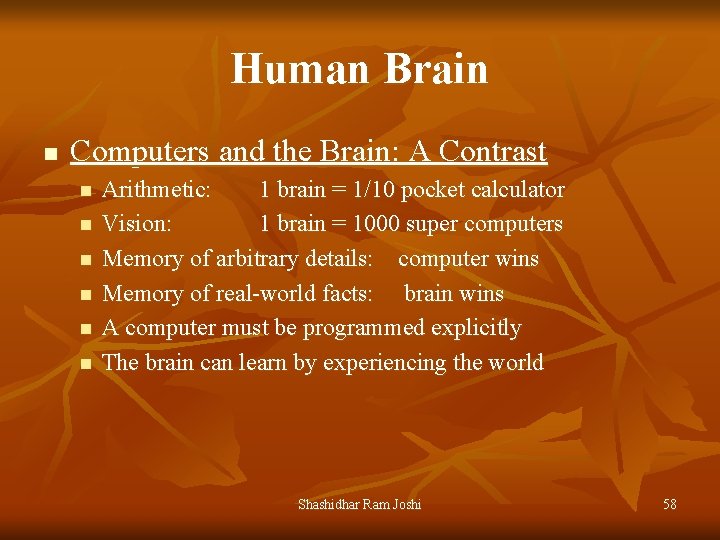
Human Brain n Computers and the Brain: A Contrast n n n Arithmetic: 1 brain = 1/10 pocket calculator Vision: 1 brain = 1000 super computers Memory of arbitrary details: computer wins Memory of real-world facts: brain wins A computer must be programmed explicitly The brain can learn by experiencing the world Shashidhar Ram Joshi 58

Definition n “. . . Neural nets are basically mathematical models of information processing. . . ” “. . . (neural nets) refer to machines that have a structure that, at some level, reflects what is known of the structure of the brain. . . ” “A neural network is a massively parallel distributed processor. . . “ Shashidhar Ram Joshi 59

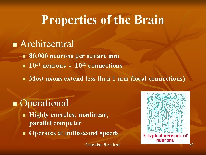
Properties of the Brain n Architectural n 80, 000 neurons per square mm 1011 neurons - 1015 connections n Most axons extend less than 1 mm (local connections) n n Operational n n Highly complex, nonlinear, parallel computer Operates at millisecond speeds Shashidhar Ram Joshi 60

Interconnectedness n n n Each neuron may have over a thousand synapses Some cells in cerebral cortex may have 200, 000 connections Total number of connections in the brain “network” is astronomical—greater than the number of particles in known universe Shashidhar Ram Joshi 61

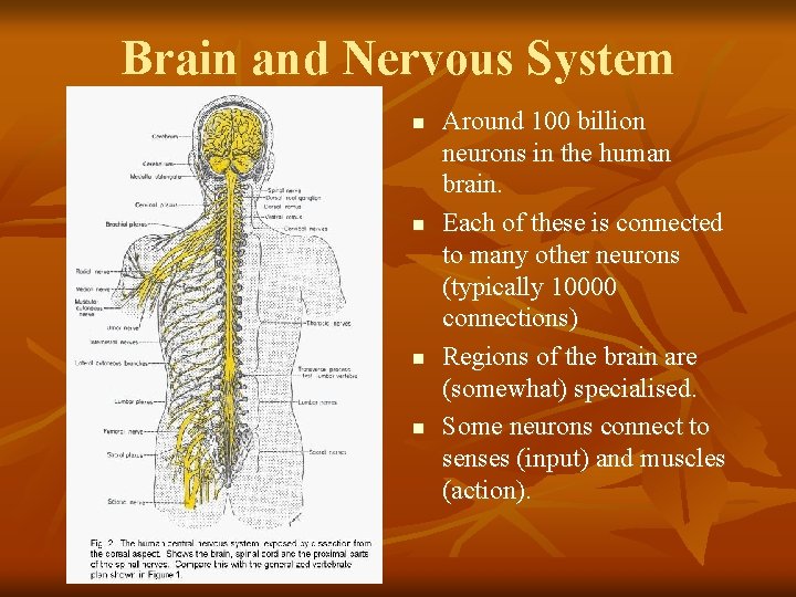
Brain and Nervous System n n Around 100 billion neurons in the human brain. Each of these is connected to many other neurons (typically 10000 connections) Regions of the brain are (somewhat) specialised. Some neurons connect to senses (input) and muscles (action).

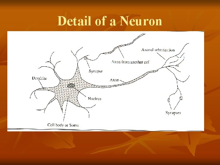
Detail of a Neuron

The Question Humans find these tasks relatively simple We learn by example The brain is responsible for our ‘computing’ power If a machine were constructed using the fundamental building blocks found in the brain could it learn to do ‘difficult’ tasks ? ? ? Shashidhar Ram Joshi 64

Basic Ideas in Machine Learning n n Machine learning is focused on inductive learning of hypotheses from examples. Three main forms of learning: n n n Supervised learning: Examples are tagged with some “expert” information. Unsupervised learning: Examples are placed into categories without guidance; instead, generic properties such as “similarity” are used. Reinforcement learning: Examples are tested, and the results of those tests used to drive learning.

Neural Network: Characteristics n n Highly parallel structure; hence a capability for fast computing Ability to learn and adapt to changing system parameters High degree of tolerance to damage in the connections Ability to learn through parallel and distributed processing 66

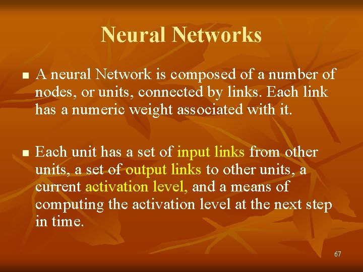
Neural Networks n n A neural Network is composed of a number of nodes, or units, connected by links. Each link has a numeric weight associated with it. Each unit has a set of input links from other units, a set of output links to other units, a current activation level, and a means of computing the activation level at the next step in time. 67

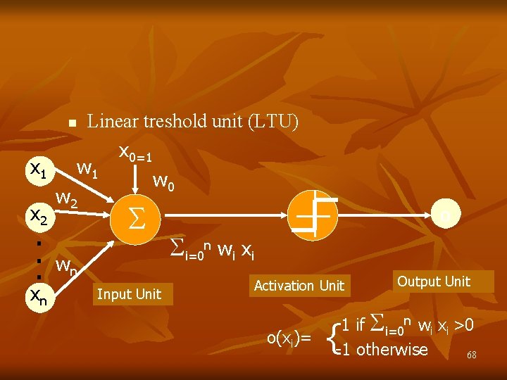
Linear treshold unit (LTU) x 0=1 w 0 n x 1 x 2 . . . xn w 2 wn Input Unit o i=0 n wi xi Activation Unit o(xi)= Output Unit 1 if i=0 n wi xi >0 -1 otherwise 68 {

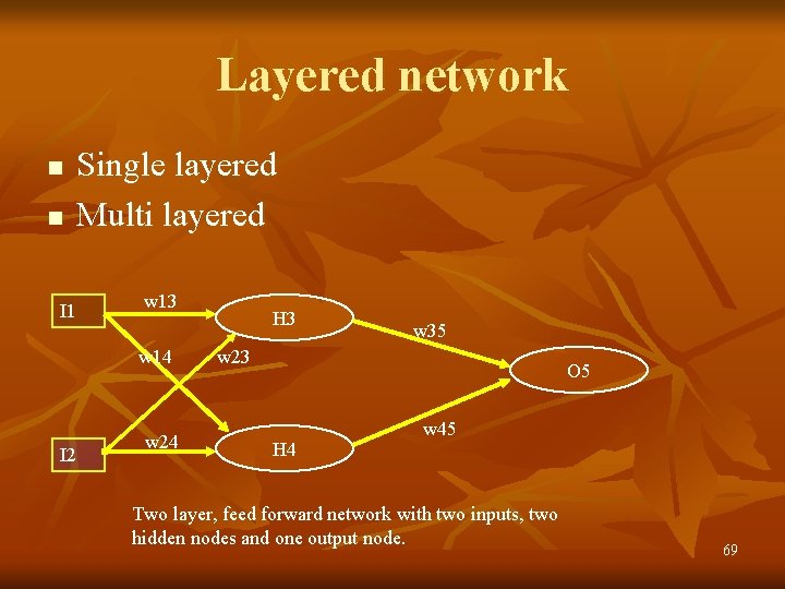
Layered network n n I 1 Single layered Multi layered w 13 w 14 I 2 w 24 H 3 w 35 w 23 O 5 H 4 w 45 Two layer, feed forward network with two inputs, two hidden nodes and one output node. 69

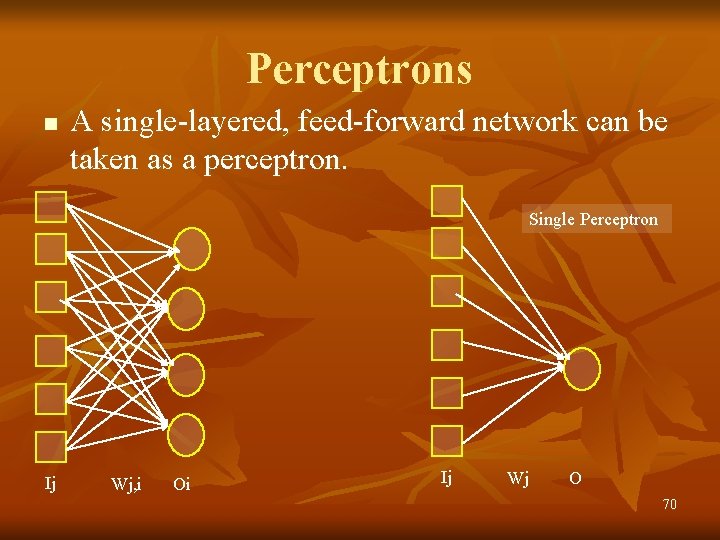
Perceptrons n A single-layered, feed-forward network can be taken as a perceptron. Single Perceptron Ij Wj, i Oi Ij Wj O 70

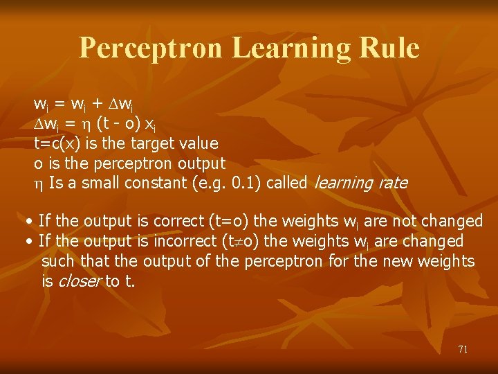
Perceptron Learning Rule wi = wi + wi wi = (t - o) xi t=c(x) is the target value o is the perceptron output Is a small constant (e. g. 0. 1) called learning rate • If the output is correct (t=o) the weights wi are not changed • If the output is incorrect (t o) the weights wi are changed such that the output of the perceptron for the new weights is closer to t. 71

Genetic Algorithm n n n Derived inspiration from biology The most fertile area for exchange of views between biology and computer science is ‘evolutionary computing’ This area evolved from three stages or less independent development: n n n Genetic algorithms Evolutionary programming Evolution strategies 74

GA. . n n The investigators began to see a strong relationship between these areas, and at present, genetic algorithms are consideered to be among the most successful machine-learning techniques. In the “origin of species”, Darwin described theory of evolution, with the ‘natural selection’ as the central notion. n n Each species has an overproduction of individuals and in a tough struggle for life, only those individuals that are best adapted to the environment survive. The long DNA molecules, consisting of only four building blocks, suggest that all the heriditary information of a human individual, or of any living creature, has been laid down in a language of only four letters (C, G, A & T in language of genetics) 75

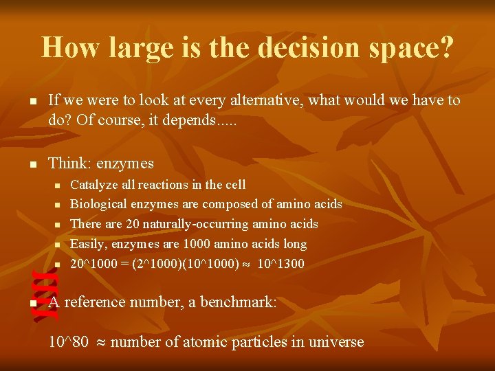
How large is the decision space? n n If we were to look at every alternative, what would we have to do? Of course, it depends. . . Think: enzymes n n n Catalyze all reactions in the cell Biological enzymes are composed of amino acids There are 20 naturally-occurring amino acids Easily, enzymes are 1000 amino acids long 20^1000 = (2^1000)(10^1000) 10^1300 A reference number, a benchmark: 10^80 number of atomic particles in universe

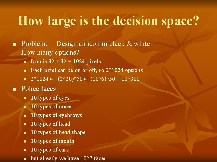
How large is the decision space? n Problem: Design an icon in black & white How many options? n n Icon is 32 x 32 = 1024 pixels Each pixel can be on or off, so 2^1024 options 2^1024 (2^20)^50 (10^6)^50 = 10^300 Police faces n n n n 10 types of eyes 10 types of noses 10 types of eyebrows 10 types of head shape 10 types of mouth 10 types of ears but already we have 10^7 faces

GA. . n The collection of genetic instruction for human is about 3 billion letters long n n Each individual inherits some characteristics of the father and some of the mother. Individual differences between people, such as hair color and eye color, and also pre-disposition for diseases, are caused by differences in genetic coding n Even the twins are different in numerous aspects. 78

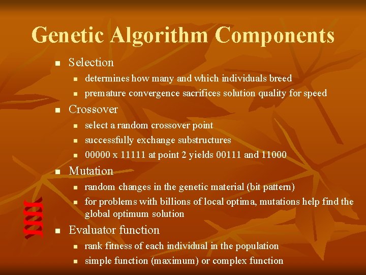
Genetic Algorithm Components n Selection n Crossover n n select a random crossover point successfully exchange substructures 00000 x 11111 at point 2 yields 00111 and 11000 Mutation n determines how many and which individuals breed premature convergence sacrifices solution quality for speed random changes in the genetic material (bit pattern) for problems with billions of local optima, mutations help find the global optimum solution Evaluator function n n rank fitness of each individual in the population simple function (maximum) or complex function

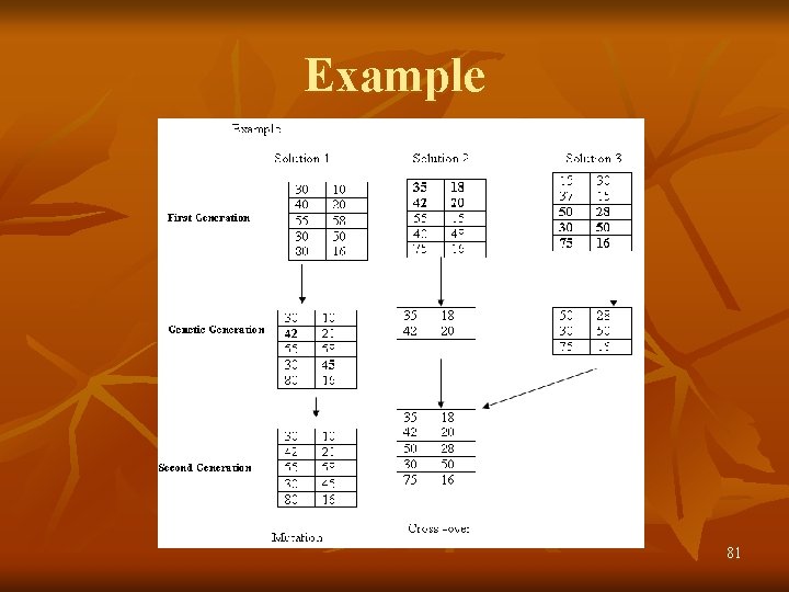
GA. . n Following are the formula for constructing a genetic algorithm for the solution of problem n n n Write a good coding in terms of strings of limited alphabets Invent an artificial environment in the computer where solution can join each other Develop ways in which possible solutions can be combined. Like father’s and mother’s strings are simply cut and after changing, stuck together again called cross- over Provide an initial population or solution set and make the computer play evolution by removing bad solutions from each generation and replacing them with mutations of good solutions Stop when a family of successful solutions has been produced 80

Example 81

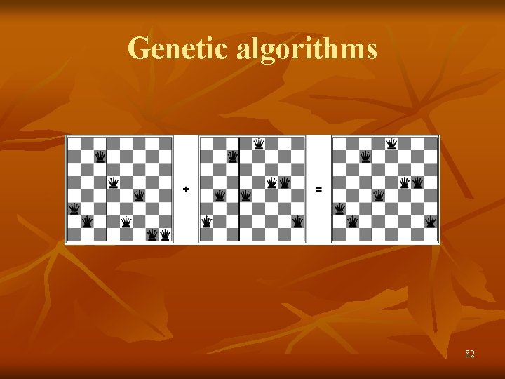
Genetic algorithms 82