Decision Procedures in First Order Logic Decision Procedures

Decision Procedures in First Order Logic Decision Procedures for Equality Logic Range Allocation Daniel Kroening and Ofer Strichman 1

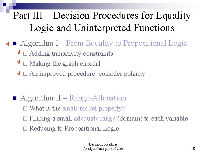
Part III – Decision Procedures for Equality Logic and Uninterpreted Functions Algorithm I – From Equality to Propositional Logic n ¨ Adding n transitivity constraints ¨ Making the graph chordal ¨ An improved procedure: consider polarity Algorithm II – Range-Allocation ¨ What is the small-model property? ¨ Finding a small adequate range (domain) to each variable ¨ Reducing to Propositional Logic Decision Procedures An algorithmic point of view 2

Range allocation n The small model property n Range Allocation Decision Procedures An algorithmic point of view 3

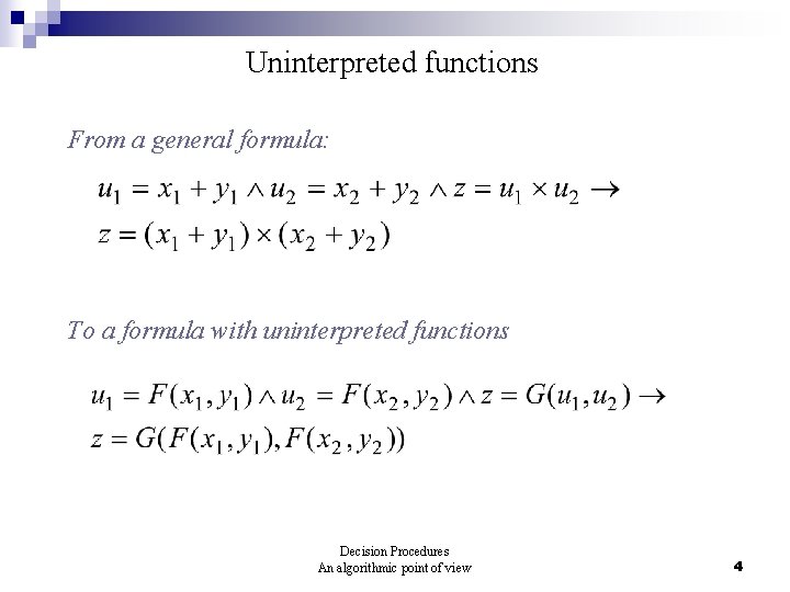
Uninterpreted functions From a general formula: To a formula with uninterpreted functions Decision Procedures An algorithmic point of view 4

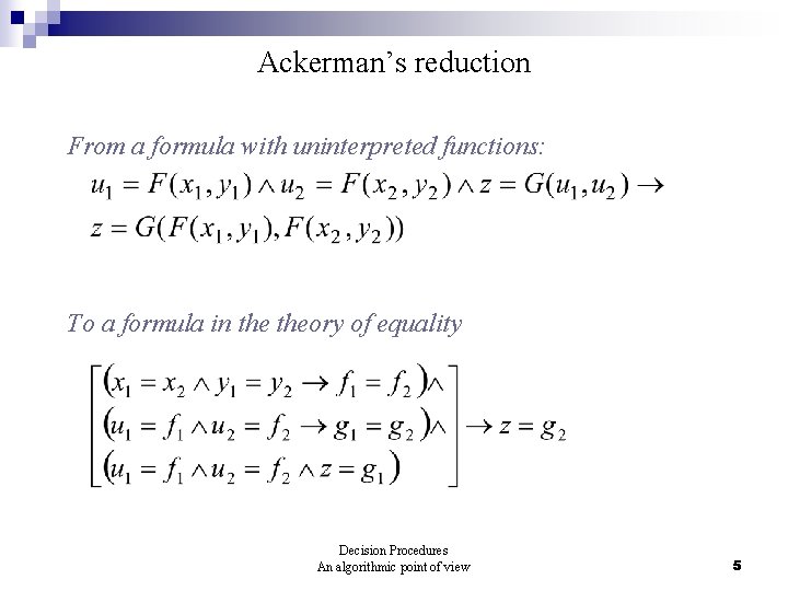
Ackerman’s reduction From a formula with uninterpreted functions: To a formula in theory of equality Decision Procedures An algorithmic point of view 5

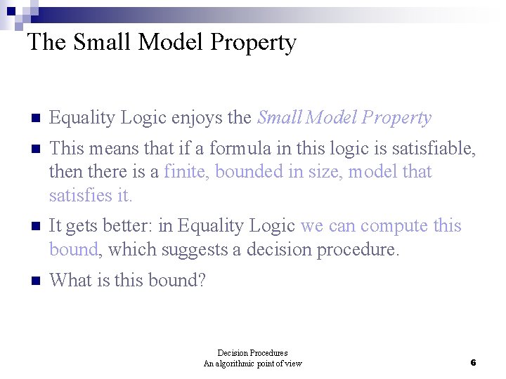
The Small Model Property n Equality Logic enjoys the Small Model Property n This means that if a formula in this logic is satisfiable, then there is a finite, bounded in size, model that satisfies it. n It gets better: in Equality Logic we can compute this bound, which suggests a decision procedure. n What is this bound? Decision Procedures An algorithmic point of view 6

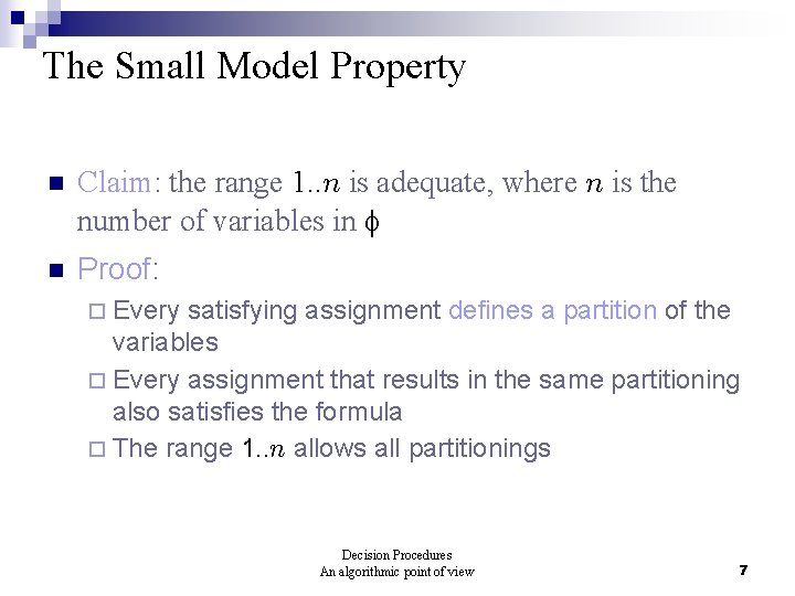
The Small Model Property n Claim: the range 1. . n is adequate, where n is the number of variables in n Proof: ¨ Every satisfying assignment defines a partition of the variables ¨ Every assignment that results in the same partitioning also satisfies the formula ¨ The range 1. . n allows all partitionings Decision Procedures An algorithmic point of view 7

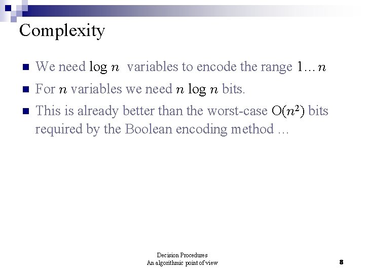
Complexity n We need log n variables to encode the range 1…n n For n variables we need n log n bits. n This is already better than the worst-case O(n 2) bits required by the Boolean encoding method … Decision Procedures An algorithmic point of view 8

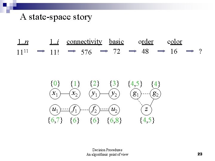
Finite Instantiations revisited Instead of giving the range [1. . 11], analyze connectivity: x 1 x 2 y 1 y 2 u 1 f 2 u 2 x 1, y 1, x 2, y 2 : {0 -1} u 1, f 2, u 2 : {0 -3} g 1 g 2 z g 1, g 2, z: {0 -2} The state-space: from 1111 to ~105 Decision Procedures An algorithmic point of view 9

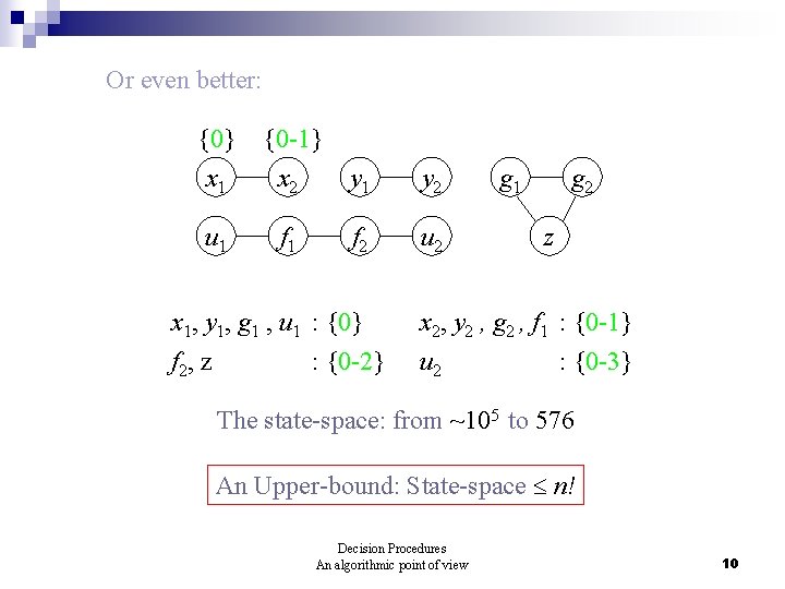
Or even better: {0} {0 -1} x 1 x 2 y 1 y 2 u 1 f 2 u 2 x 1, y 1, g 1 , u 1 : {0} f 2, z : {0 -2} g 1 g 2 z x 2, y 2 , g 2 , f 1 : {0 -1} u 2 : {0 -3} The state-space: from ~105 to 576 An Upper-bound: State-space n! Decision Procedures An algorithmic point of view 10

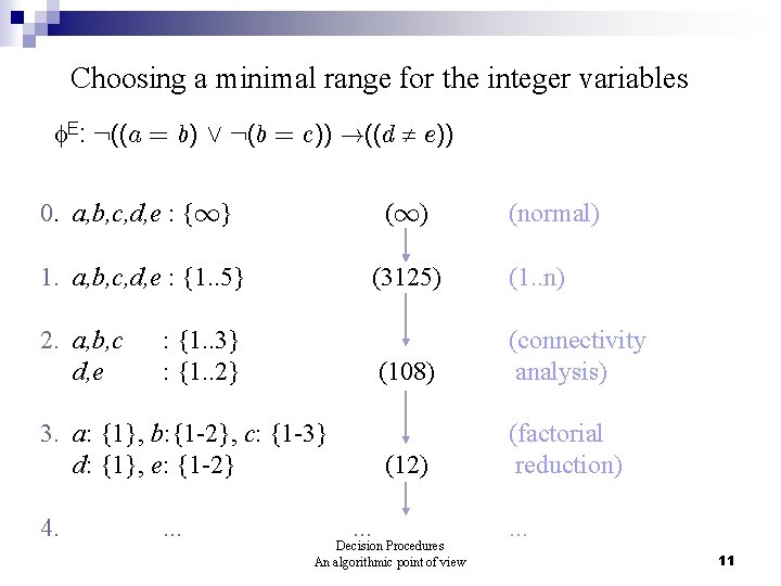
Choosing a minimal range for the integer variables E: : ((a = b) Ç : (b = c)) !((d e)) 0. a, b, c, d, e : {1} (1) 1. a, b, c, d, e : {1. . 5} (3125) (1. . n) (108) (connectivity analysis) (12) (factorial reduction) 2. a, b, c d, e : {1. . 3} : {1. . 2} 3. a: {1}, b: {1 -2}, c: {1 -3} d: {1}, e: {1 -2} 4. . . . Decision Procedures An algorithmic point of view (normal) . . . 11

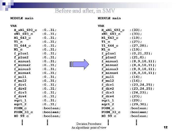
Before and after, in SMV Decision Procedures An algorithmic point of view 12

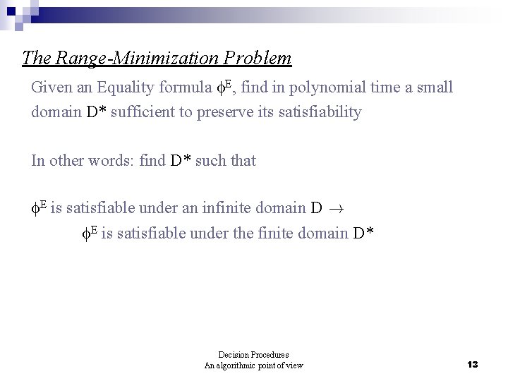
The Range-Minimization Problem Given an Equality formula E, find in polynomial time a small domain D* sufficient to preserve its satisfiability In other words: find D* such that E is satisfiable under an infinite domain D ! E is satisfiable under the finite domain D* Decision Procedures An algorithmic point of view 13

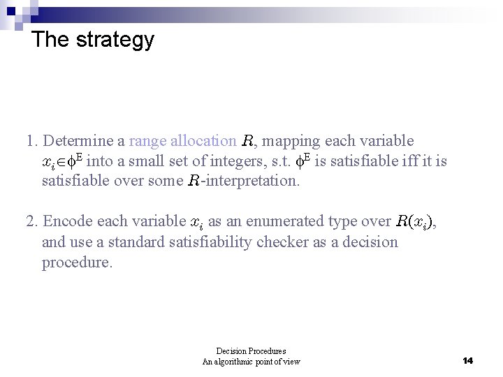
The strategy 1. Determine a range allocation R, mapping each variable xi E into a small set of integers, s. t. E is satisfiable iff it is satisfiable over some R-interpretation. 2. Encode each variable xi as an enumerated type over R(xi), and use a standard satisfiability checker as a decision procedure. Decision Procedures An algorithmic point of view 14

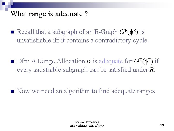
What range is adequate ? n Recall that a subgraph of an E-Graph GE( E) is unsatisfiable iff it contains a contradictory cycle. n Dfn: A Range Allocation R is adequate for GE( E) if every satisfiable subgraph can be satisfied under R. n Now we need an algorithm to find adequate ranges Decision Procedures An algorithmic point of view 15

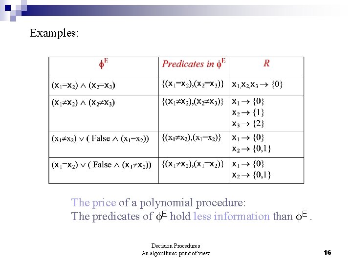
Examples: The price of a polynomial procedure: The predicates of E hold less information than E. Decision Procedures An algorithmic point of view 16

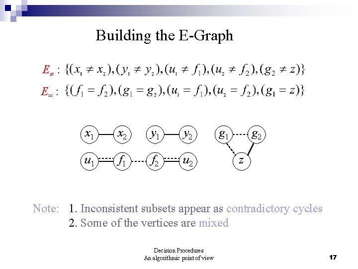
Building the E-Graph E : E= : x 1 x 2 y 1 y 2 u 1 f 2 u 2 g 1 g 2 z Note: 1. Inconsistent subsets appear as contradictory cycles 2. Some of the vertices are mixed Decision Procedures An algorithmic point of view 17

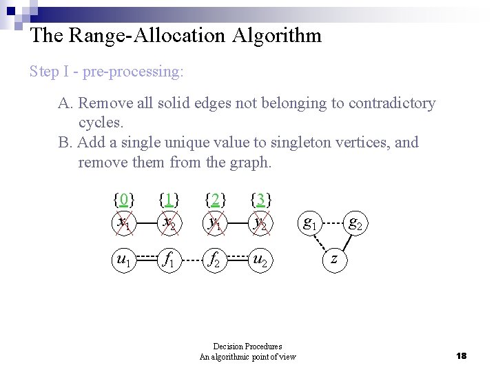
The Range-Allocation Algorithm Step I - pre-processing: A. Remove all solid edges not belonging to contradictory cycles. B. Add a single unique value to singleton vertices, and remove them from the graph. {0} x 1 {1} x 2 {2} y 1 {3} y 2 u 1 f 2 u 2 Decision Procedures An algorithmic point of view g 1 g 2 z 18

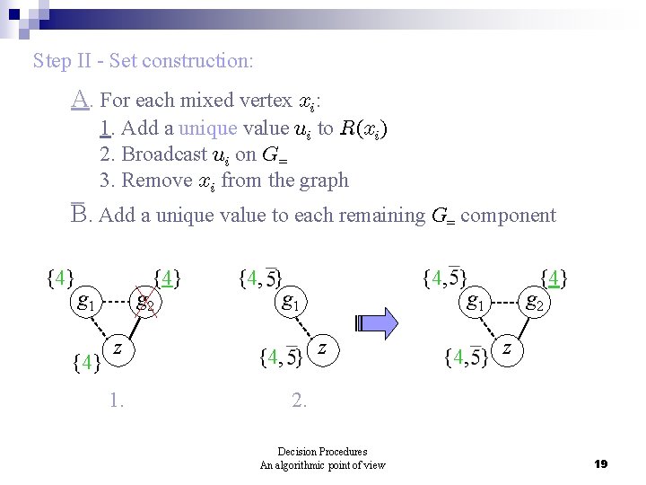
Step II - Set construction: A. For each mixed vertex xi: 1. Add a unique value ui to R(xi) 2. Broadcast ui on G= 3. Remove xi from the graph B. Add a unique value to each remaining G= component {4} g 1 {4} g 2 z 1. {4, } g 1 {4, } z {4, } g 1 {4} g 2 {4, } z 2. Decision Procedures An algorithmic point of view 19

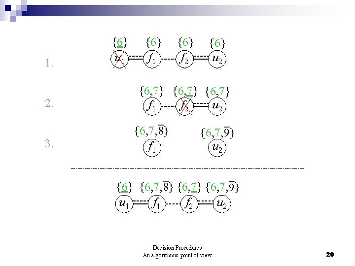
1. 2. 3. {6} u 1 {6} f 2 {6} u 2 {6, 7} f 1 f 2 u 2 {6, 7, } f 1 {6, 7, } u 2 {6} {6, 7, } u 1 f 2 u 2 Decision Procedures An algorithmic point of view 20

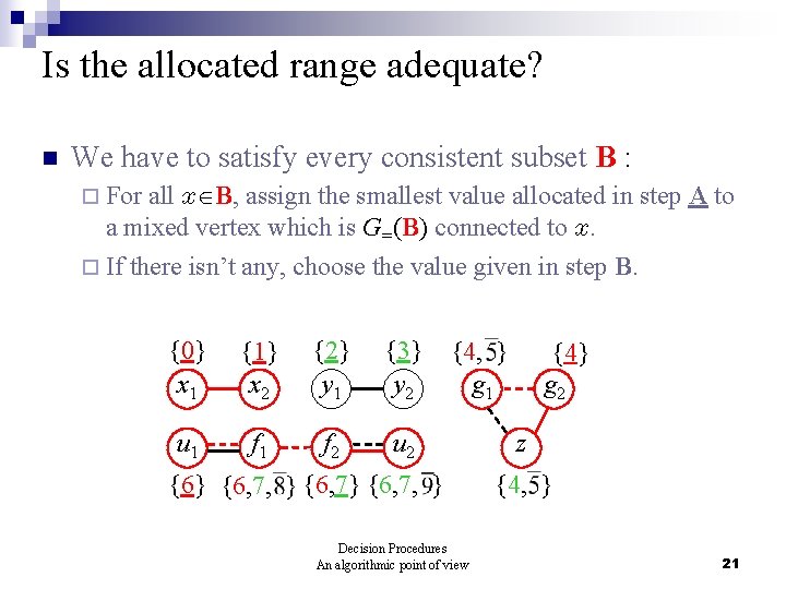
Is the allocated range adequate? n We have to satisfy every consistent subset B : ¨ For all x B, assign the smallest value allocated in step A to a mixed vertex which is G=(B) connected to x. ¨ If there isn’t any, choose the value given in step B. {0} x 1 {1} x 2 {2} y 1 {3} y 2 u 1 f 2 u 2 {4, } g 1 {6} {6, 7, } Decision Procedures An algorithmic point of view {4} g 2 z {4, } 21

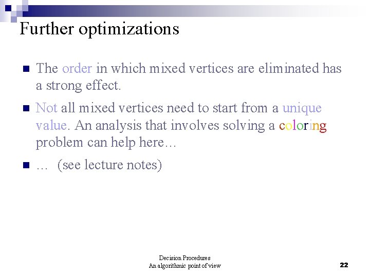
Further optimizations n The order in which mixed vertices are eliminated has a strong effect. n Not all mixed vertices need to start from a unique value. An analysis that involves solving a coloring problem can help here… n … (see lecture notes) Decision Procedures An algorithmic point of view 22

A state-space story 1. . n 1. . i 1111 11! connectivity basic 72 576 {0} x 1 {1} x 2 {2} y 1 {3} y 2 u 1 f 2 u 2 {6, 7} {6} order 48 {4, 5} g 1 {6} {6, 8} Decision Procedures An algorithmic point of view color 16 ? {4} g 2 z {4, 5} 23