Decision Procedures for Equality Logic and Uninterpreted Functions

Decision Procedures for Equality Logic and Uninterpreted Functions Daniel Kroening and Ofer Strichman Decision Procedure 1/66 Decision Procedure Changki Hong @ PSWLAB

Last talk. . We learnt about Equality logic and Equality logic with uninterpreted functions. There were two reduction schemes to transform Equality logic with uninterpreted functions into Equality logic. Today, we will cover how to determine satisfiability of the Equality logic. 2/66 Decision Procedure Changki Hong @ PSWLAB

Contents Decision procedure for the Equality logic and UFs Decision procedure for the Equality logic Transform equality logic to propositional logic Range allocation algorithm 3/66 Decision Procedure Changki Hong @ PSWLAB

Basic assumptions and notations Assumptions Input formulas are in NNF (Negation Normal Form) Input formulas are checked for satisfiability Notations Equality formula with Uninterpreted Functions: UF Equality formula: E 4/66 Decision Procedure Changki Hong @ PSWLAB

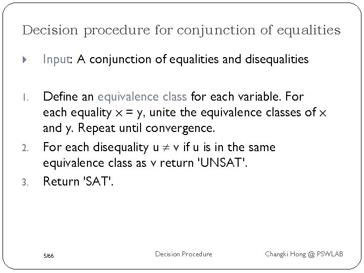
Decision procedure for conjunction of equalities Input: A conjunction of equalities and disequalities 1. Define an equivalence class for each variable. For each equality x = y, unite the equivalence classes of x and y. Repeat until convergence. For each disequality u v if u is in the same equivalence class as v return 'UNSAT'. Return 'SAT'. 2. 3. 5/66 Decision Procedure Changki Hong @ PSWLAB

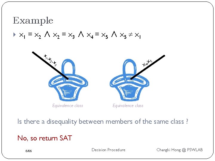
Example x 1 = x 2 ∧ x 2 = x 3 ∧ x 4 = x 5 ∧ x 5 x 1 , x 2 , x 3 Equivalence class x 4, x 5 Equivalence class Is there a disequality between members of the same class ? No, so return SAT 6/66 Decision Procedure Changki Hong @ PSWLAB

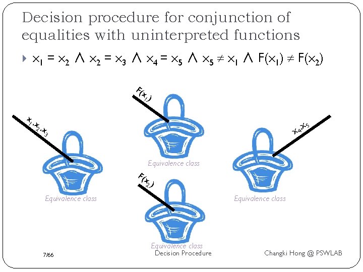
Decision procedure for conjunction of equalities with uninterpreted functions x 1 = x 2 ∧ x 2 = x 3 ∧ x 4 = x 5 ∧ x 5 x 1 ∧ F(x 1) F(x 2) F(x 1) x 1 , x 2 , x 4, x 3 x 5 Equivalence class F(x 2) Equivalence class 7/66 Decision Procedure Changki Hong @ PSWLAB

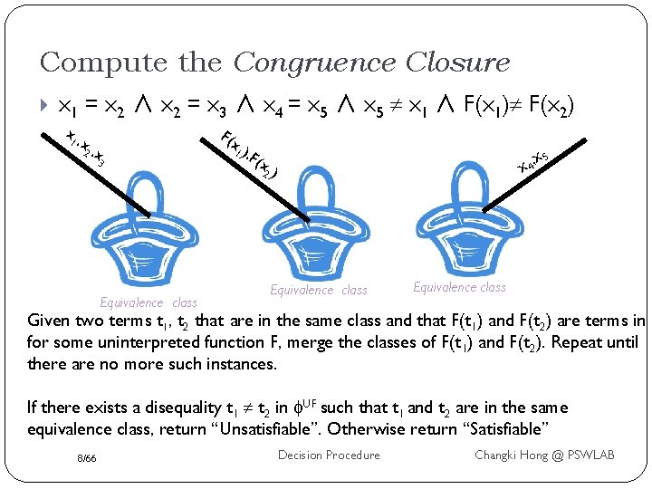
Compute the Congruence Closure x 1 = x 2 ∧ x 2 = x 3 ∧ x 4 = x 5 ∧ x 5 x 1 ∧ F(x 1) F(x 2) x 1 , x 2 , x 3 Equivalence class F(x 1 ), F (x x 4, 2) Equivalence class x 5 Equivalence class Given two terms t 1, t 2 that are in the same class and that F(t 1) and F(t 2) are terms in for some uninterpreted function F, merge the classes of F(t 1) and F(t 2). Repeat until there are no more such instances. If there exists a disequality t 1 t 2 in UF such that t 1 and t 2 are in the same equivalence class, return “Unsatisfiable”. Otherwise return “Satisfiable” 8/66 Decision Procedure Changki Hong @ PSWLAB

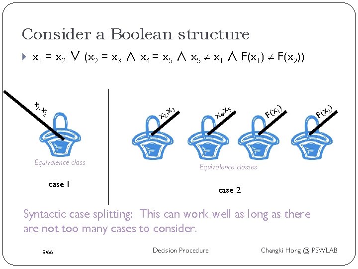
Consider a Boolean structure x 1 = x 2 ∨ (x 2 = x 3 ∧ x 4 = x 5 ∧ x 5 x 1 ∧ F(x 1) F(x 2)) x 1 , x 2 x 5 x 4, x 3 x 2, Equivalence class ) 1 x ( F ) 2 x ( F Equivalence classes case 1 case 2 Syntactic case splitting: This can work well as long as there are not too many cases to consider. 9/66 Decision Procedure Changki Hong @ PSWLAB

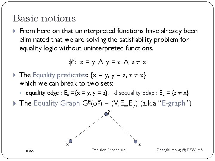
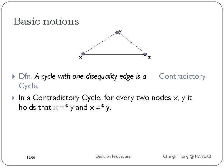
Basic notions From here on that uninterpreted functions have already been eliminated that we are solving the satisfiability problem for equality logic without uninterpreted functions. E: x = y ∧ y = z ∧ z x The Equality predicates: {x = y, y = z, z x} which we can break to two sets: equality edge : E= ={x = y, y = z}, disequality edge : E = {z x} The Equality Graph GE( E) = (V, E=, E ) (a. k. a “E-graph”) y x 10/66 z Decision Procedure Changki Hong @ PSWLAB

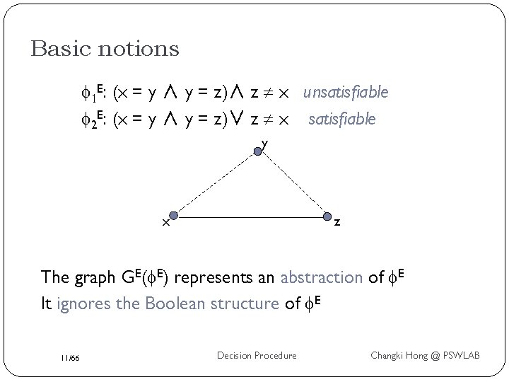
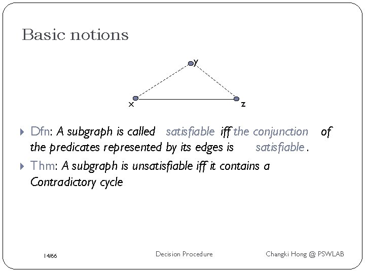
Basic notions 1 E: (x = y ∧ y = z)∧ z x unsatisfiable 2 E: (x = y ∧ y = z)∨ z x satisfiable y x z The graph GE( E) represents an abstraction of E It ignores the Boolean structure of E 11/66 Decision Procedure Changki Hong @ PSWLAB

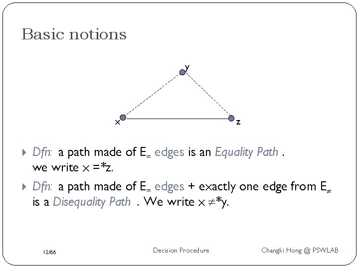
Basic notions y x z Dfn: a path made of E= edges is an Equality Path. we write x =*z. Dfn: a path made of E= edges + exactly one edge from E is a Disequality Path. We write x *y. 12/66 Decision Procedure Changki Hong @ PSWLAB

Basic notions y x z Dfn. A cycle with one disequality edge is a Contradictory Cycle. In a Contradictory Cycle, for every two nodes x, y it holds that x =* y and x * y. 13/66 Decision Procedure Changki Hong @ PSWLAB

Basic notions y x z Dfn: A subgraph is called satisfiable iff the conjunction of the predicates represented by its edges is satisfiable. Thm: A subgraph is unsatisfiable iff it contains a Contradictory cycle 14/66 Decision Procedure Changki Hong @ PSWLAB

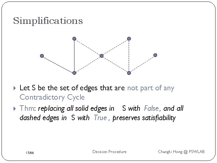
Simplifications Let S be the set of edges that are not part of any Contradictory Cycle Thm: replacing all solid edges in S with False , and all dashed edges in S with True , preserves satisfiability 15/66 Decision Procedure Changki Hong @ PSWLAB

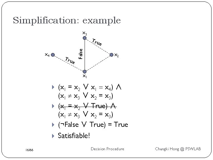
Simplification: example x 3 Tru x 4 Tru e False e x 2 x 1 (x 1 = x 2 ∨ x 1 = x 4) ∧ (x 1 x 3 ∨ x 2 = x 3) (x 1 = x 2 ∨ True) ∧ (x 1 x 3 ∨ x 2 = x 3) (¬False ∨ True) = True Satisfiable! 16/66 Decision Procedure Changki Hong @ PSWLAB

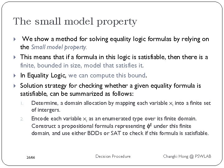
Decision procedures for Equality logic and UFs From hereon we are going to look at algorithms which transform Equality logic into propositional logic and use decision procedure for propositional logic. Algorithm I – From Equality to Propositional Logic Adding transitivity constraints Making the graph chordal Algorithm II – Range-Allocation What is the small-model property? Finding a small adequate range (domain) to each variable Reducing to Propositional Logic 17/66 Decision Procedure Changki Hong @ PSWLAB

Decision Procedures for Equality Logic We will first investigate methods that solve Equality Logic. Uninterpreted functions are eliminated with one of the reduction schemes. Our starting point: the E-Graph GE( E) Recall that GE( E) represents an abstraction of E. It represents ALL equality formulas with the same set of equality predicates as E. 18/66 Decision Procedure Changki Hong @ PSWLAB

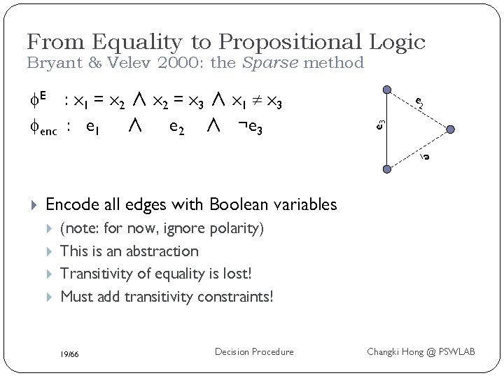
From Equality to Propositional Logic Bryant & Velev 2000: the Sparse method e 2 e 3 E : x 1 = x 2 ∧ x 2 = x 3 ∧ x 1 x 3 enc : e 1 ∧ e 2 ∧ ¬e 3 e 1 Encode all edges with Boolean variables (note: for now, ignore polarity) This is an abstraction Transitivity of equality is lost! Must add transitivity constraints! 19/66 Decision Procedure Changki Hong @ PSWLAB

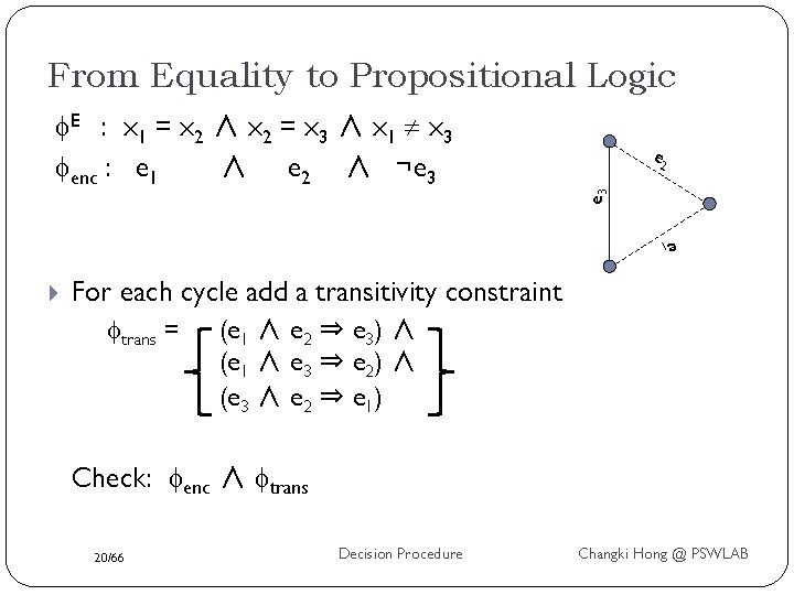
From Equality to Propositional Logic E : x 1 = x 2 ∧ x 2 = x 3 ∧ x 1 x 3 enc : e 1 ∧ e 2 ∧ ¬e 3 e 2 e 1 For each cycle add a transitivity constraint trans = (e 1 ∧ e 2 ⇒ e 3) ∧ (e 1 ∧ e 3 ⇒ e 2) ∧ (e 3 ∧ e 2 ⇒ e 1) Check: enc ∧ trans 20/66 Decision Procedure Changki Hong @ PSWLAB

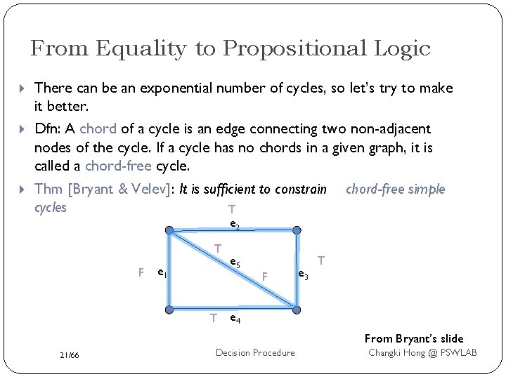
From Equality to Propositional Logic There can be an exponential number of cycles, so let’s try to make it better. Dfn: A chord of a cycle is an edge connecting two non-adjacent nodes of the cycle. If a cycle has no chords in a given graph, it is called a chord-free cycle. Thm [Bryant & Velev]: It is sufficient to constrain chord-free simple cycles T e 2 T F e 1 e 5 F e 3 T T e 4 From Bryant’s slide 21/66 Decision Procedure Changki Hong @ PSWLAB

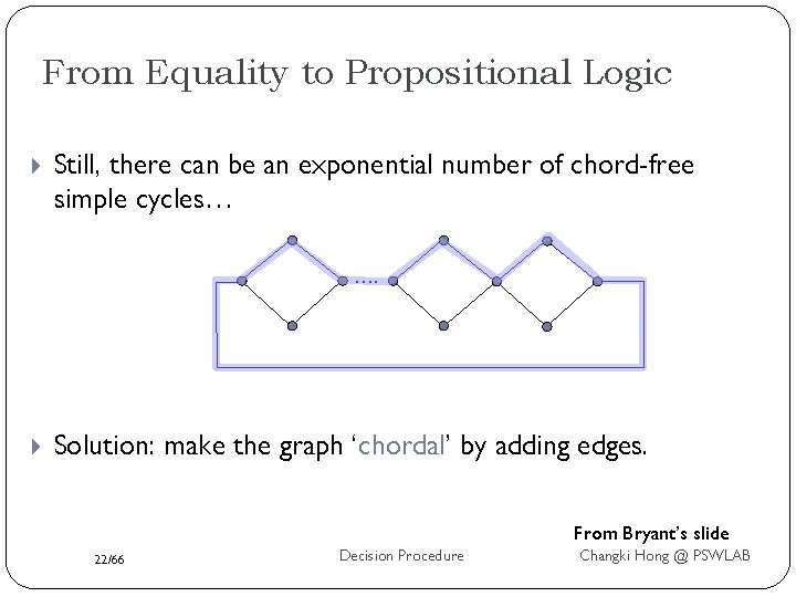
From Equality to Propositional Logic Still, there can be an exponential number of chord-free simple cycles… …. Solution: make the graph ‘chordal’ by adding edges. From Bryant’s slide 22/66 Decision Procedure Changki Hong @ PSWLAB

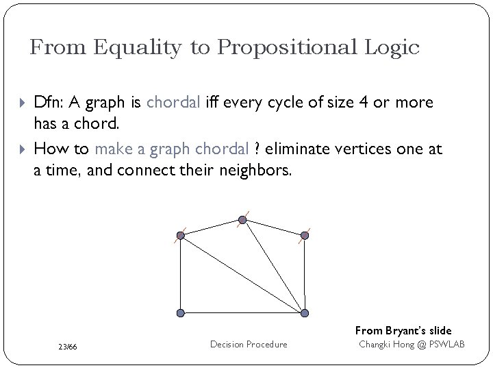
From Equality to Propositional Logic Dfn: A graph is chordal iff every cycle of size 4 or more has a chord. How to make a graph chordal ? eliminate vertices one at a time, and connect their neighbors. From Bryant’s slide 23/66 Decision Procedure Changki Hong @ PSWLAB

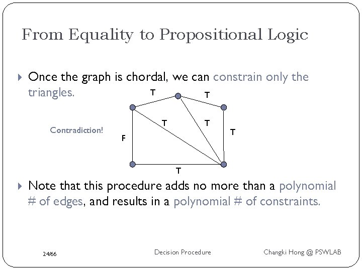
From Equality to Propositional Logic Once the graph is chordal, we can constrain only the T triangles. T Contradiction! T T F T T Note that this procedure adds no more than a polynomial # of edges, and results in a polynomial # of constraints. 24/66 Decision Procedure Changki Hong @ PSWLAB

Decision Procedures for Equality logic and UFs Algorithm I – From Equality to Propositional Logic Adding transitivity constraints Making the graph chordal Algorithm II – Range-Allocation Small-model property Finding a small adequate range (domain) to each variable Reducing to Propositional Logic 25/66 Decision Procedure Changki Hong @ PSWLAB

The small model property We show a method for solving equality logic formulas by relying on the Small model property. This means that if a formula in this logic is satisfiable, then there is a finite, bounded in size, model that satisfies it. In Equality Logic, we can compute this bound. Solution strategy for checking whether a given equality formula is satisfiable, can be summarized as follows: 1. 2. Determine, a domain allocation by mapping each variable xi into a finite set of intergers. Encode each variable xi as an enumerated type over its finite domain. Construct a propositional formula representing E under this finite domain, and use either BDDs or SAT to check if this formula is satisfiable. 26/66 Decision Procedure Changki Hong @ PSWLAB

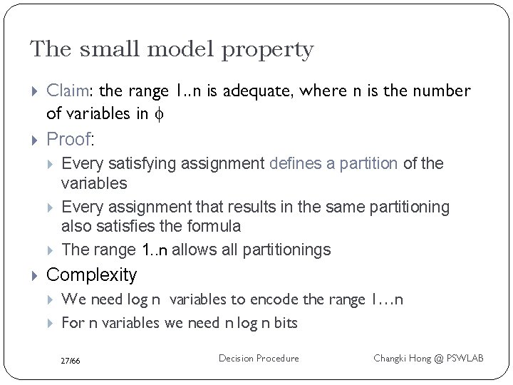
The small model property Claim: the range 1. . n is adequate, where n is the number of variables in Proof: Every satisfying assignment defines a partition of the variables Every assignment that results in the same partitioning also satisfies the formula The range 1. . n allows all partitionings Complexity We need log n variables to encode the range 1…n For n variables we need n log n bits 27/66 Decision Procedure Changki Hong @ PSWLAB

Reducing state-space Instead of giving the range [1. . 11], analyze connectivity: x 1 x 2 y 1 y 2 u 1 f 2 u 2 x 1, y 1, x 2, y 2 : {0 -1} u 1, f 2, u 2 : {0 -3} g 1 g 2 z g 1, g 2, z: {0 -2} The state-space: from 1111 to ~ 110592 28/66 Decision Procedure Changki Hong @ PSWLAB

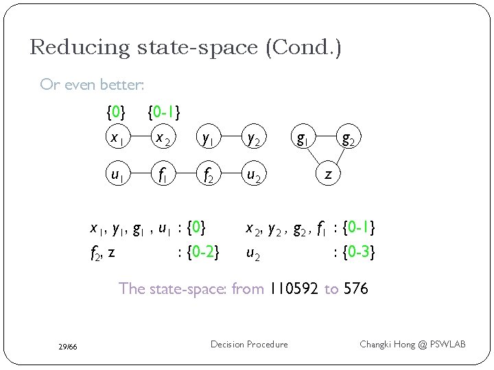
Reducing state-space (Cond. ) Or even better: {0} x 1 {0 -1} x 2 y 1 y 2 u 1 f 2 u 2 x 1, y 1, g 1 , u 1 : {0} f 2, z : {0 -2} g 1 g 2 z x 2, y 2 , g 2 , f 1 : {0 -1} u 2 : {0 -3} The state-space: from 110592 to 576 29/66 Decision Procedure Changki Hong @ PSWLAB

Range minimization problem Given an Equality formula E, find in polynomial time a small domain D* sufficient to preserve its satisfiability In other words: find D* such that E is satisfiable under an infinite domain D → E is satisfiable under the finite domain D* 30/66 Decision Procedure Changki Hong @ PSWLAB

The strategy 1. Determine a range allocation R, mapping each variable xi E into a small set of integers, such that E is satisfiable iff it is satisfiable over some R-interpretation. 2. Encode each variable xi as an enumerated type over R(xi), and use a standard satisfiability checker as a decision procedure. 31/66 Decision Procedure Changki Hong @ PSWLAB

What range is adequate ? Recall that a subgraph of an E-Graph GE( E) is unsatisfiable iff it contains a contradictory cycle. Dfn: A Range Allocation R is adequate for GE( E) if every satisfiable subgraph can be satisfied under R. Now we need an algorithm to find adequate ranges 32/66 Decision Procedure Changki Hong @ PSWLAB

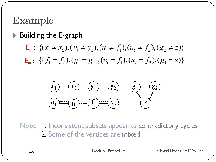
Example Building the E-graph E : E= : x 1 x 2 y 1 y 2 u 1 f 2 u 2 g 1 g 2 z Note: 1. Inconsistent subsets appear as contradictory cycles 2. Some of the vertices are mixed 33/66 Decision Procedure Changki Hong @ PSWLAB

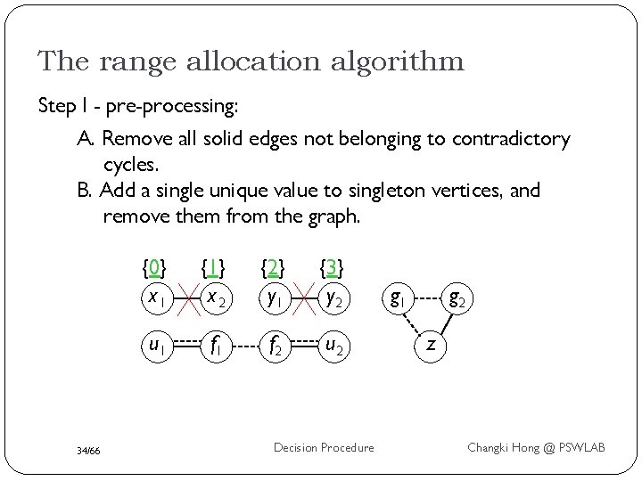
The range allocation algorithm Step I - pre-processing: A. Remove all solid edges not belonging to contradictory cycles. B. Add a single unique value to singleton vertices, and remove them from the graph. 34/66 {0} x 1 {1} x 2 {2} y 1 {3} y 2 u 1 f 2 u 2 Decision Procedure g 1 g 2 z Changki Hong @ PSWLAB

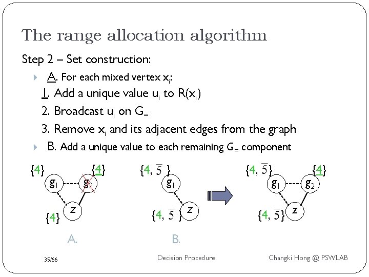
The range allocation algorithm Step 2 – Set construction: A. For each mixed vertex xi: 1. Add a unique value ui to R(xi) 2. Broadcast ui on G= 3. Remove xi and its adjacent edges from the graph B. Add a unique value to each remaining G = component {4} g 1 {4} g 2 z A. 35/66 {4, } g 1 {4, } g 1 }z {4} g 2 {4, } z B. Decision Procedure Changki Hong @ PSWLAB

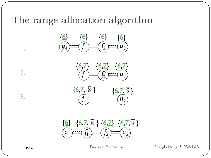
The range allocation algorithm 1. 2. 3. {6} u 1 {6} f 1 {6} u 2 {6, 7} f 1 f 2 u 2 {6, 7, f 1 {6} {6, 7, u 1 f 1 36/66 {6} f 2 } {6, 7, } u 2 } {6, 7, } f 2 u 2 Decision Procedure Changki Hong @ PSWLAB

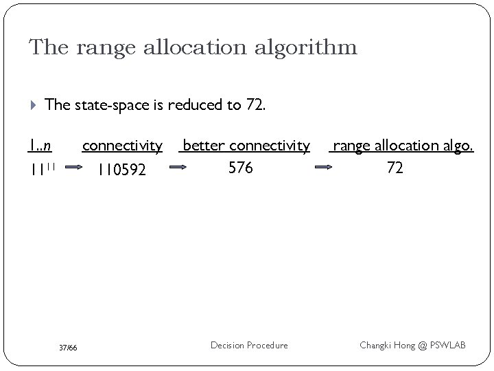
The range allocation algorithm The state-space is reduced to 72. 1. . n 1111 connectivity 110592 37/66 better connectivity 576 Decision Procedure range allocation algo. 72 Changki Hong @ PSWLAB

Conclusion Decision procedure for the equality logic with UFs, which uses syntactic case splitting method, is inefficient if the formula has many disjunctions. There are two algorithms which transform the original equality logic formula into the corresponding propositional logic formula and then check satisfiability using BDDs or SAT solver. 38/66 Decision Procedure Changki Hong @ PSWLAB

Linear Arithmetic Daniel Kroening and Ofer Strichman Decision Procedure 39/66 Decision Procedure Changki Hong @ PSWLAB

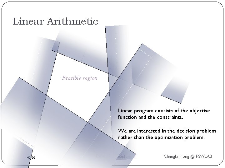
Linear Arithmetic Feasible region Linear program consists of the objective function and the constraints. We are interested in the decision problem rather than the optimization problem. 40/66 Decision Procedure Changki Hong @ PSWLAB

Simplex algorithm The simplex algorithm is developed by Danzig in 1947 but it still efficiently used. The simplex algorithm can decide satisfiability of a conjunction of linear inequalities. The set of constraints is normally accompanied by a linear objective functions in terms of the variables of the formula. If the set of constraints is satisfiable, the simplex algorithm provides a satisfying assignment that maximizes the value of the objective function. As we are concerned with the decision problem rather than the optimization problem, we are going to cover a variant of the simplex algo. called general simplex that does not require an objective function. 41/66 Decision Procedure Changki Hong @ PSWLAB

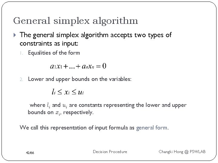
General simplex algorithm The general simplex algorithm accepts two types of constraints as input: 1. Equalities of the form 2. Lower and upper bounds on the variables: where li and ui are constants representing the lower and upper bounds on xi, respectively. We call this representation of input formula as general form. 42/66 Decision Procedure Changki Hong @ PSWLAB

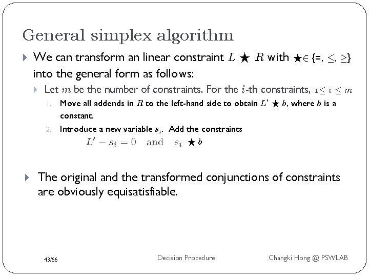
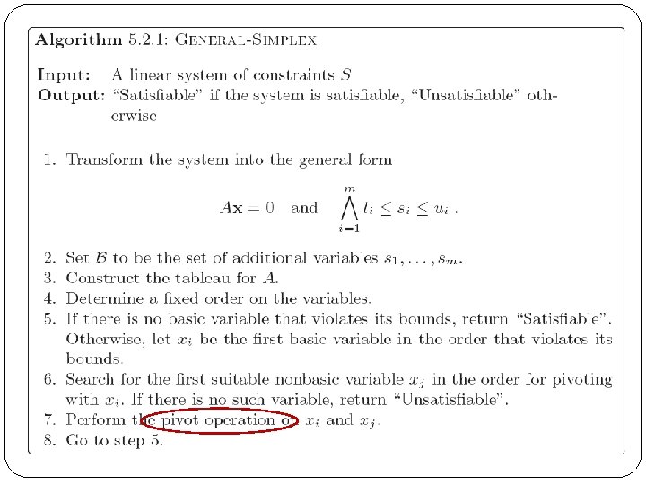
General simplex algorithm We can transform an linear constraint L F R with F 2 {=, ·, ¸} into the general form as follows: Let m be the number of constraints. For the i-th constraints, 1· i · m 1. 2. Move all addends in R to the left-hand side to obtain L’ F b, where b is a constant. Introduce a new variable si. Add the constraints Fb The original and the transformed conjunctions of constraints are obviously equisatisfiable. 43/66 Decision Procedure Changki Hong @ PSWLAB

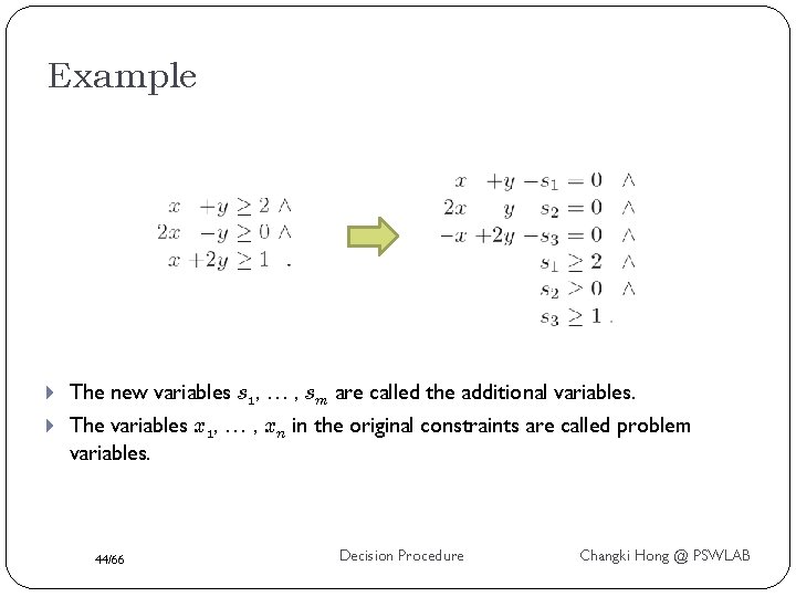
Example The new variables s 1, … , sm are called the additional variables. The variables x 1, … , xn in the original constraints are called problem variables. 44/66 Decision Procedure Changki Hong @ PSWLAB

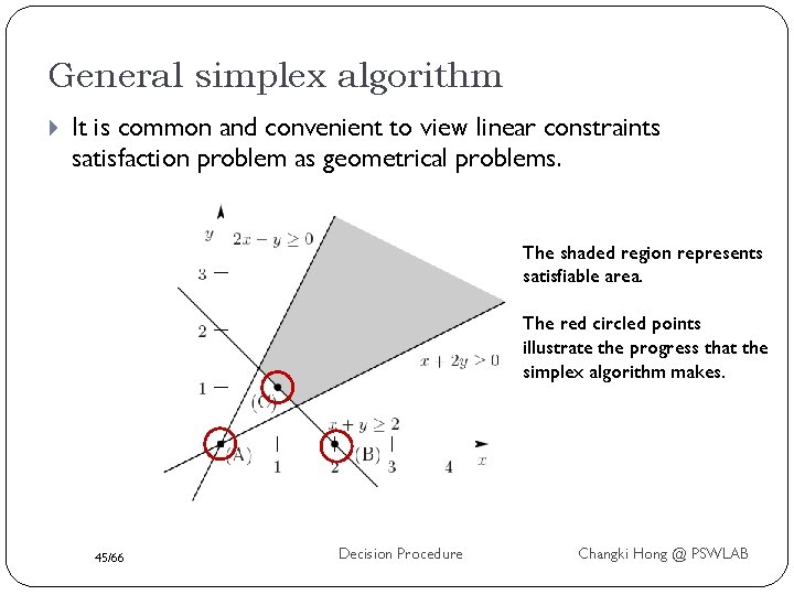
General simplex algorithm It is common and convenient to view linear constraints satisfaction problem as geometrical problems. The shaded region represents satisfiable area. The red circled points illustrate the progress that the simplex algorithm makes. 45/66 Decision Procedure Changki Hong @ PSWLAB

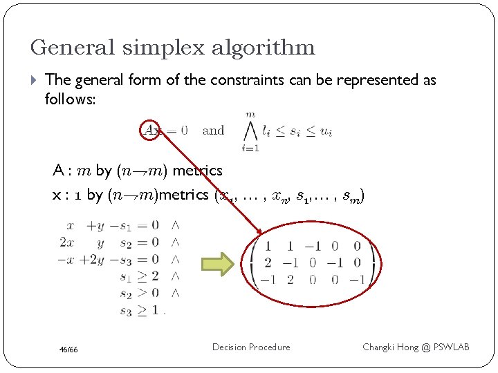
General simplex algorithm The general form of the constraints can be represented as follows: A : m by (n+m) metrics x : 1 by (n+m)metrics (x 1, … , xn, s 1, … , sm) 46/66 Decision Procedure Changki Hong @ PSWLAB

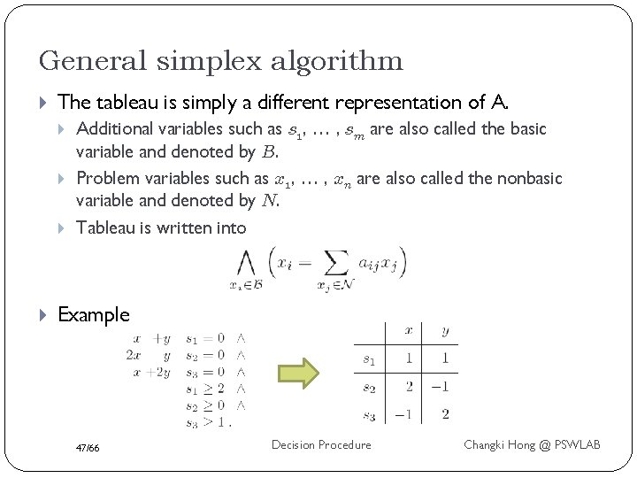
General simplex algorithm The tableau is simply a different representation of A. Additional variables such as s 1, … , sm are also called the basic variable and denoted by B. Problem variables such as x 1, … , xn are also called the nonbasic variable and denoted by N. Tableau is written into Example 47/66 Decision Procedure Changki Hong @ PSWLAB

General simplex algorithm 48/66 Decision Procedure Changki Hong @ PSWLAB

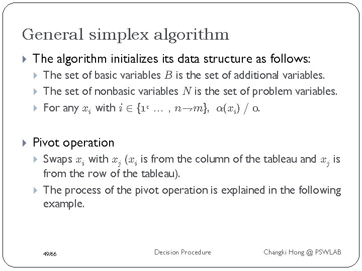
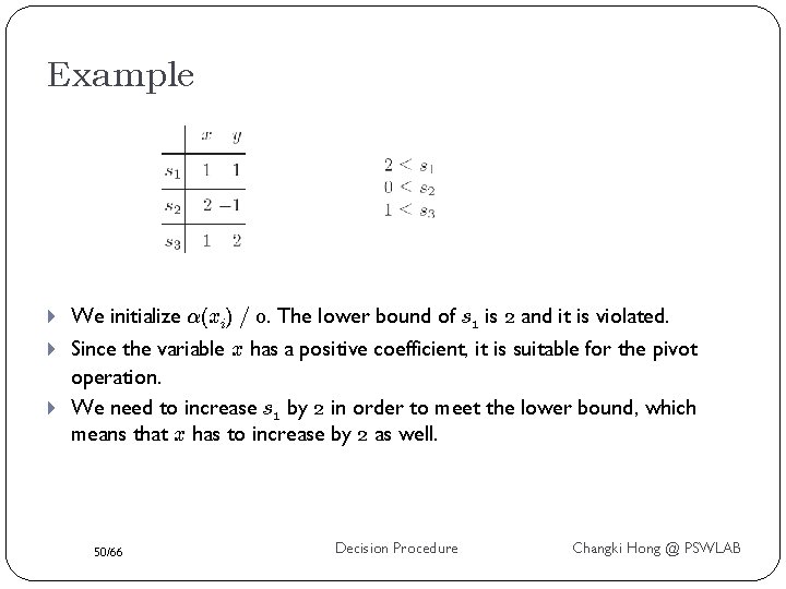
General simplex algorithm The algorithm initializes its data structure as follows: The set of basic variables B is the set of additional variables. The set of nonbasic variables N is the set of problem variables. For any xi with i 2 {1, … , n+m}, ®(xi) = 0. Pivot operation Swaps xi with xj (xi is from the column of the tableau and xj is from the row of the tableau). The process of the pivot operation is explained in the following example. 49/66 Decision Procedure Changki Hong @ PSWLAB

Example We initialize ®(xi) = 0. The lower bound of s 1 is 2 and it is violated. Since the variable x has a positive coefficient, it is suitable for the pivot operation. We need to increase s 1 by 2 in order to meet the lower bound, which means that x has to increase by 2 as well. 50/66 Decision Procedure Changki Hong @ PSWLAB

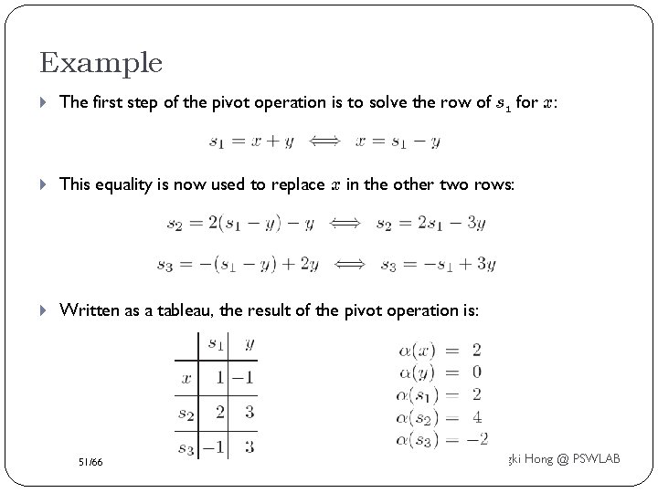
Example The first step of the pivot operation is to solve the row of s 1 for x: This equality is now used to replace x in the other two rows: Written as a tableau, the result of the pivot operation is: 51/66 Decision Procedure Changki Hong @ PSWLAB

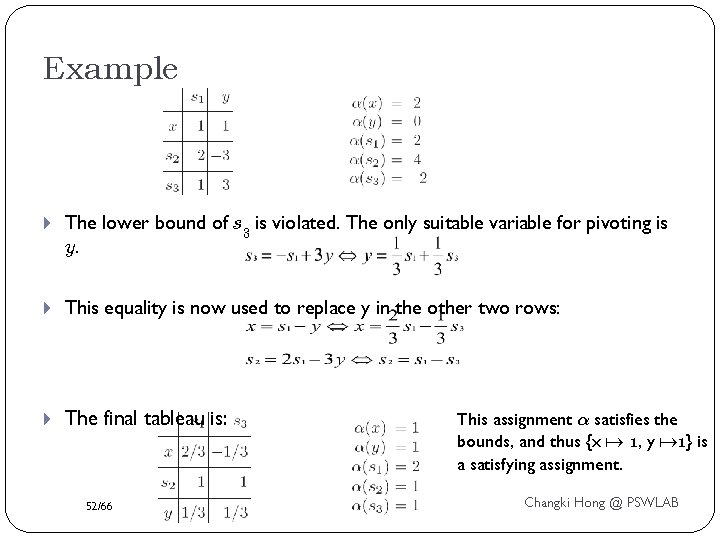
Example The lower bound of s 3 is violated. The only suitable variable for pivoting is y. This equality is now used to replace y in the other two rows: The final tableau is: 52/66 This assignment ® satisfies the bounds, and thus {x 1, y 1} is a satisfying assignment. Decision Procedure Changki Hong @ PSWLAB

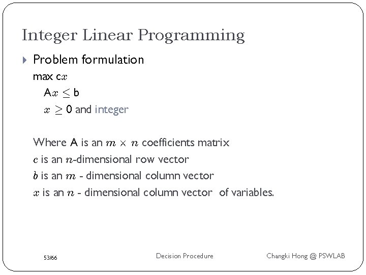
Integer Linear Programming Problem formulation max cx Ax · b x ¸ 0 and integer Where A is an m £ n coefficients matrix c is an n-dimensional row vector b is an m - dimensional column vector x is an n - dimensional column vector of variables. 53/66 Decision Procedure Changki Hong @ PSWLAB

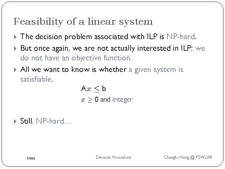
Feasibility of a linear system The decision problem associated with ILP is NP-hard. But once again, we are not actually interested in ILP: we do not have an objective function. All we want to know is whether a given system is satisfiable. Ax · b x ¸ 0 and integer Still, NP-hard… 54/66 Decision Procedure Changki Hong @ PSWLAB

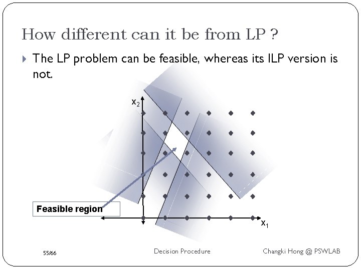
How different can it be from LP ? The LP problem can be feasible, whereas its ILP version is not. x 2 Feasible region x 1 55/66 Decision Procedure Changki Hong @ PSWLAB

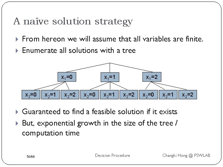
A naïve solution strategy From hereon we will assume that all variables are finite. Enumerate all solutions with a tree x 1=0 x 2=0 x 2=1 x 2=2 x 1=1 x 2=0 x 2=1 x 2=2 Guaranteed to find a feasible solution if it exists But, exponential growth in the size of the tree / computation time 56/66 Decision Procedure Changki Hong @ PSWLAB

A family of algorithms: Branch & Bound Probably the most popular method for solving Integer Linear Programming (ILP) problems (First presented in 1960) is B & B. It is the optimization problem. However, we are interested in deciding feasibility of a linear system. 57/66 Decision Procedure Changki Hong @ PSWLAB

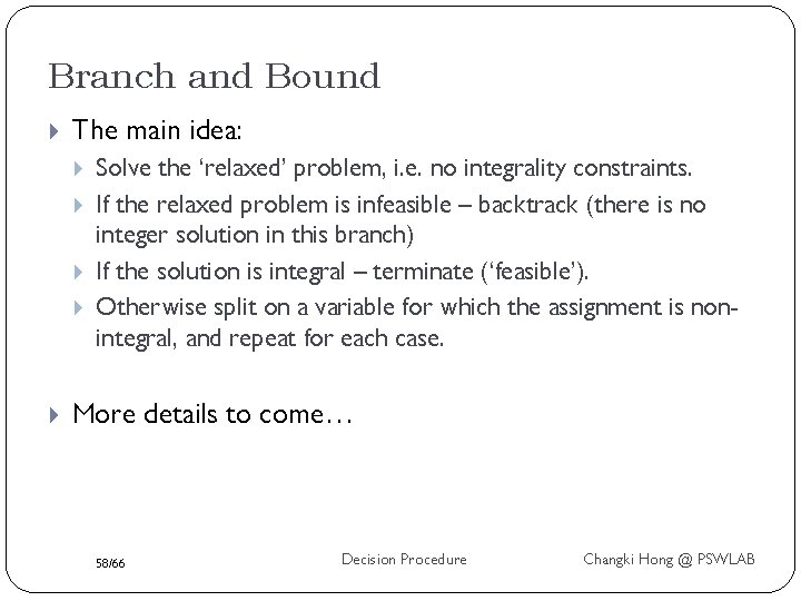
Branch and Bound The main idea: Solve the ‘relaxed’ problem, i. e. no integrality constraints. If the relaxed problem is infeasible – backtrack (there is no integer solution in this branch) If the solution is integral – terminate (‘feasible’). Otherwise split on a variable for which the assignment is nonintegral, and repeat for each case. More details to come… 58/66 Decision Procedure Changki Hong @ PSWLAB

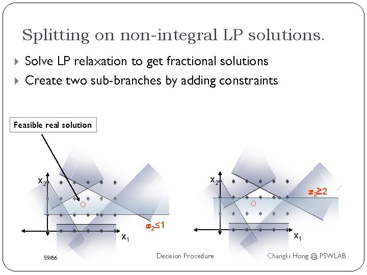
Splitting on non-integral LP solutions. Solve LP relaxation to get fractional solutions Create two sub-branches by adding constraints Feasible real solution x 2 x 2≥ 2 x 1 59/66 x 2≤ 1 Decision Procedure x 1 Changki Hong @ PSWLAB

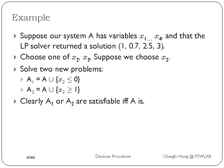
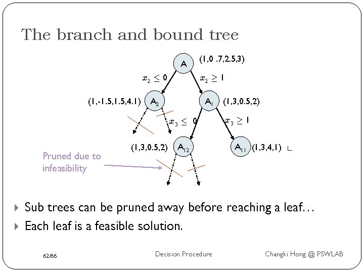
Example Suppose our system A has variables x 1… x 4, and that the LP solver returned a solution (1, 0. 7, 2. 5, 3). Choose one of x 2, x 3. Suppose we choose x 2. Solve two new problems: A 1 = A [ {x 2 · 0} A 2 = A [ {x 2 ¸ 1} Clearly A 1 or A 2 are satisfiable iff A is. 60/66 Decision Procedure Changki Hong @ PSWLAB

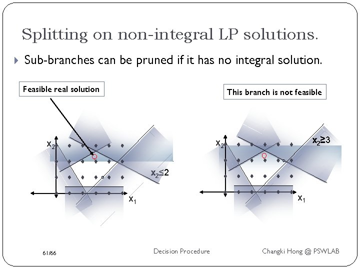
Splitting on non-integral LP solutions. Sub-branches can be pruned if it has no integral solution. Feasible real solution This branch is not feasible x 2≥ 3 x 2 x 2≤ 2 x 1 61/66 Decision Procedure Changki Hong @ PSWLAB

The branch and bound tree A x 2 · 0 (1, -1. 5, 4. 1) (1, 0. 7, 2. 5, 3) x 2 ¸ 1 A 2 A 1 x 3 · 0 Pruned due to infeasibility (1, 3, 0. 5, 2) A 12 (1, 3, 0. 5, 2) x 3 ¸ 1 A 11 (1, 3, 4, 1) x Sub trees can be pruned away before reaching a leaf… Each leaf is a feasible solution. 62/66 Decision Procedure Changki Hong @ PSWLAB

Conclusion General simplex algorithm can check satisfiability of LP constraints. ILP is NP-hard but Branch and bound algorithm works efficiently in practice. 63/66 Decision Procedure Changki Hong @ PSWLAB