Decision Models Lecture 5 1 Lecture 5 Integer

Decision Models Lecture 5 1 Lecture 5 Integer Programming 4 Plant-location example m Portfolio Optimization – Part I 4 The Scenario Approach 4 The Mean-Variance Model m Summary and Preparation for next class m

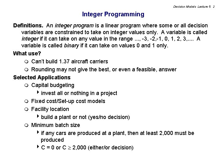
Decision Models Lecture 5 2 Integer Programming Definitions. An integer program is a linear program where some or all decision variables are constrained to take on integer values only. A variable is called integer if it can take on any value in the range. . . , -3, -2, -1, 0, 1, 2, 3, . . A variable is called binary if it can take on values 0 and 1 only. What use? m Can’t build 1. 37 aircraft carriers m Rounding may not give the best, or even a feasible, answer Selected Applications m Capital budgeting 4 invest all or nothing in a project m Fixed cost/Set-up cost models m Facility location 4 build a plant or not (yes/no decision) m Minimum batch size 4 if any cars are produced at a plant, then at least 2, 000 must be produced 4 C = 0 or C 2, 000 (either/or decision)

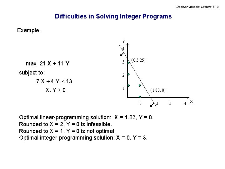
Decision Models Lecture 5 3 Difficulties in Solving Integer Programs Example. Y 4 max 21 X + 11 Y subject to: 7 X + 4 Y 13 X, Y 0 3 (0, 3. 25) 2 1 (1. 83, 0) 1 Optimal linear-programming solution: X = 1. 83, Y = 0. Rounded to X = 2, Y = 0 is infeasible. Rounded to X = 1, Y = 0 is not optimal. Optimal integer-programming solution: X = 0, Y = 3. 2 3 4 X

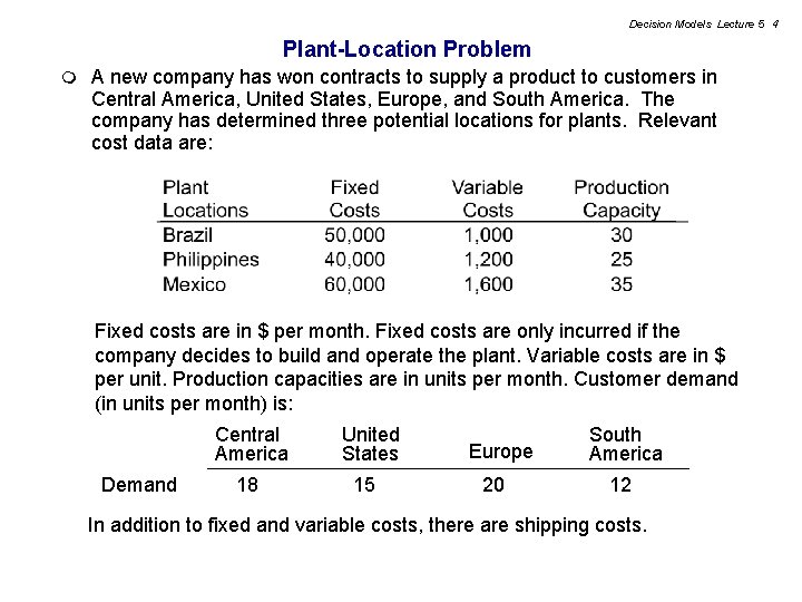
Decision Models Lecture 5 4 Plant-Location Problem m A new company has won contracts to supply a product to customers in Central America, United States, Europe, and South America. The company has determined three potential locations for plants. Relevant cost data are: Fixed costs are in $ per month. Fixed costs are only incurred if the company decides to build and operate the plant. Variable costs are in $ per unit. Production capacities are in units per month. Customer demand (in units per month) is: Central America Demand 18 United States 15 Europe 20 South America 12 In addition to fixed and variable costs, there are shipping costs.

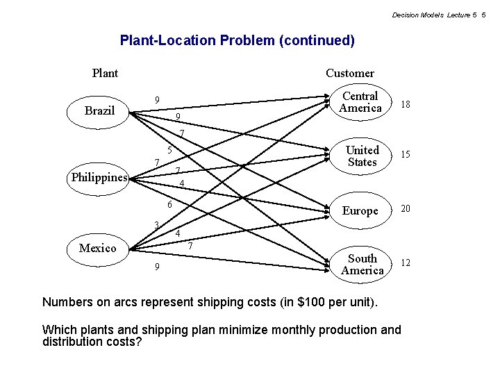
Decision Models Lecture 5 5 Plant-Location Problem (continued) Plant Brazil Customer 9 9 Central America 18 United States 15 Europe 20 South America 12 7 5 7 7 4 Philippines 6 3 4 7 Mexico 9 Numbers on arcs represent shipping costs (in $100 per unit). Which plants and shipping plan minimize monthly production and distribution costs?

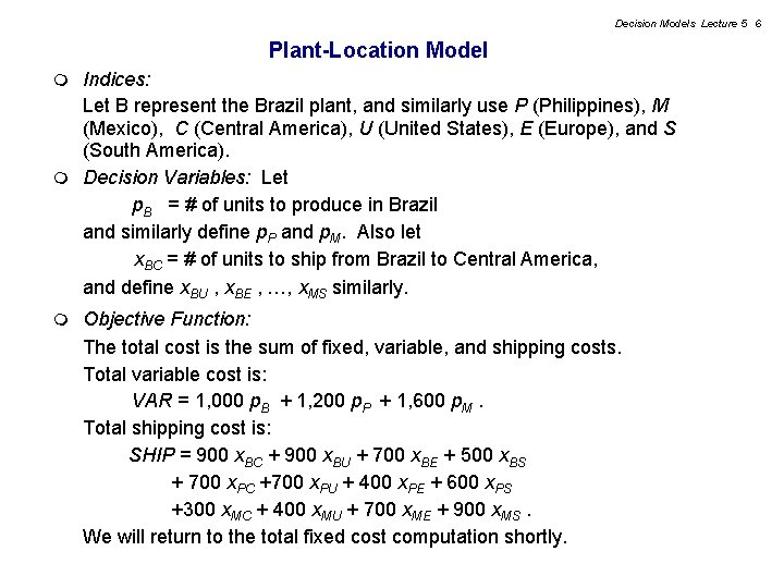
Decision Models Lecture 5 6 Plant-Location Model Indices: Let B represent the Brazil plant, and similarly use P (Philippines), M (Mexico), C (Central America), U (United States), E (Europe), and S (South America). m Decision Variables: Let p. B = # of units to produce in Brazil and similarly define p. P and p. M. Also let x. BC = # of units to ship from Brazil to Central America, and define x. BU , x. BE , …, x. MS similarly. m m Objective Function: The total cost is the sum of fixed, variable, and shipping costs. Total variable cost is: VAR = 1, 000 p. B + 1, 200 p. P + 1, 600 p. M. Total shipping cost is: SHIP = 900 x. BC + 900 x. BU + 700 x. BE + 500 x. BS + 700 x. PC +700 x. PU + 400 x. PE + 600 x. PS +300 x. MC + 400 x. MU + 700 x. ME + 900 x. MS. We will return to the total fixed cost computation shortly.

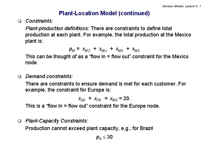
Decision Models Lecture 5 7 Plant-Location Model (continued) m Constraints: Plant-production definitions: There are constraints to define total production at each plant. For example, the total production at the Mexico plant is: p. M = x. MC + x. MU + x. ME + x. MS This can be thought of as a “flow in = flow out” constraint for the Mexico node. m Demand constraints: There are constraints to ensure demand is met for each customer. For example, the constraint for Europe is: x. BE + x. PE + x. ME = 20. This is a “flow in = flow out” constraint for the Europe node. m Plant-Capacity Constraints: Production cannot exceed plant capacity, e. g. , for Brazil p. B 30

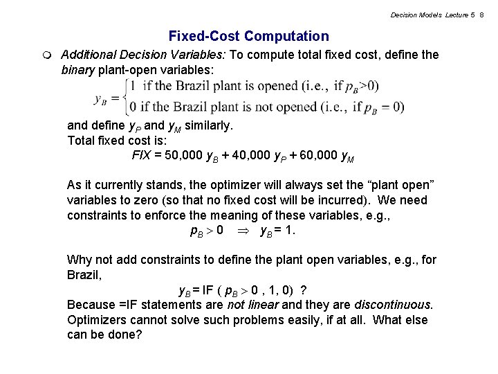
Decision Models Lecture 5 8 Fixed-Cost Computation m Additional Decision Variables: To compute total fixed cost, define the binary plant-open variables: and define y. P and y. M similarly. Total fixed cost is: FIX = 50, 000 y. B + 40, 000 y. P + 60, 000 y. M As it currently stands, the optimizer will always set the “plant open” variables to zero (so that no fixed cost will be incurred). We need constraints to enforce the meaning of these variables, e. g. , p. B 0 y. B = 1. Why not add constraints to define the plant open variables, e. g. , for Brazil, y. B = IF ( p. B 0 , 1, 0) ? Because =IF statements are not linear and they are discontinuous. Optimizers cannot solve such problems easily, if at all. What else can be done?

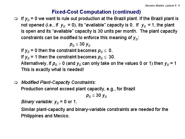
Decision Models Lecture 5 9 Fixed-Cost Computation (continued) m If y. B = 0 we want to rule out production at the Brazil plant. If the Brazil plant is not opened (i. e. , if y. B = 0), its “available” capacity is 0. If y. B = 1, the plant is open and its “available” capacity is 30 units per month. The plant capacity constraints can be modified to enforce this meaning of y. B: p. B 30 y. B If y. B = 0 then the constraint becomes p. B 0. If y. B = 1 then the constraint becomes p. B 30. Alternatively, if p. B 0 (and y. B can only take on the values 0 or 1) then y. B = 1 This is exactly what is needed! m Modified Plant-Capacity Constraints: Production cannot exceed plant capacity, e. g. , for Brazil p. B 30 y. B Binary variable: y. B = 0 or 1. Similar plant-capacity and binary-variable constraints are needed for the Philippines and Mexico.

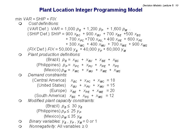
Decision Models Lecture 5 10 Plant Location Integer Programming Model min VAR + SHIP + FIX m m m Cost definitions: (VAR Def. ) VAR = 1, 000 p. B + 1, 200 p. P + 1, 600 p. M. (SHIP Def. ) SHIP = 900 x. BC + 900 x. BU + 700 x. BE +500 x. BS + 700 x. PC +700 x. PU, + 400 x. PE + 600 x. PS + 300 x. MC + 400 x. MU + 700 x. ME + 900 x. MS (FIX Def. ) FIX = 50, 000 y. B + 40, 000 y. P + 60, 000 y. M Plant production definitions: (Brazil) p. B = x. BC + x. BU + x. BE + x. BS (Philippines) p. P = x. PC + x. PU + x. PE + x. PS (Mexico) p. M = x. MC + x. MU + x. ME + x. MS Demand constraints: (Central America) x. BC + x. PC + x. MC = 18 (United States) x. BU + x. PU + x. MU = 15 (Europe) x. BE + x. PE + x. ME = 20 (South America) x. BS + x. PS + x. MS = 12 Modified plant capacity constraints: (Brazil) p. B 30 y. B (Philippines) p. P 25 y. P (Mexico) p. M 35 y. M Binary variables: y. B , y. P , y. M = 0 or 1 Nonnegativity: All variables 0

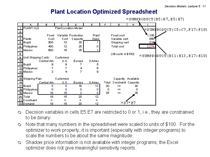
Decision Models Lecture 5 11 Plant Location Optimized Spreadsheet =SUMPRODUCT(B 5: B 7, E 5: E 7) A 1 2 3 4 5 6 PLANT. XLS Plants Brazil Philippines 7 Mexico 8 9 10 11 12 13 14 15 16 17 18 19 20 21 22 B C D E F G H Plant Location Model Fixed Cost 500 400 600 Variable Production Cost Capacity 10 30 12 25 16 35 I =SUMPRODUCT(C 5: C 7, F 17: F 19) Plant Open 1 0 1 Fixed cost Variable cost Shipping cost Total cost (All costs in $100) Unit Shipping Costs: Customers Central Am. U. S. Brazil 9 9 Philippines 7 7 Mexico 3 4 Europe 7 4 7 S. Amer. 5 6 9 Shipping Plan: Customers Central Am. U. S. Brazil 0 0 Philippines 0 0 Mexico 18 15 Total 18 15 Constraint = = 15 Demand 18 Europe 18 0 2 20 = 20 S. Amer. 12 0 0 12 = 12 1, 100 860 314 2, 274 =SUMPRODUCT(B 11: E 13, B 17: E 19) Capacity Available Total Constraint Capacity 30 <= 30 0 <= 0 35 <= 35 =D 7*E 7 Decision variables in cells E 5: E 7 are restricted to 0 or 1, i. e. , they are constrained to be binary. m Note that many numbers in the spreadsheet were scaled to units of $100. For the optimizer to work properly, it is important (especially with integer programs) to scale the numbers to be about the same magnitude. m Shadow price information is not available with integer programs; the Excel optimizer does not give meaningful sensitivity reports. m

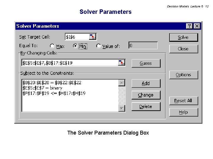
Decision Models Lecture 5 12 Solver Parameters The Solver Parameters Dialog Box

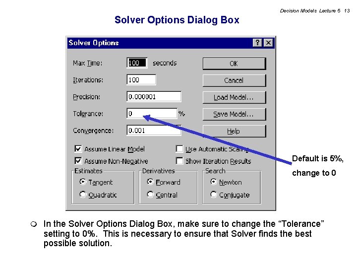
Decision Models Lecture 5 13 Solver Options Dialog Box Default is 5%, change to 0 m In the Solver Options Dialog Box, make sure to change the “Tolerance” setting to 0%. This is necessary to ensure that Solver finds the best possible solution.

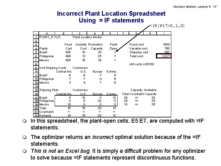
Decision Models Lecture 5 14 Incorrect Plant Location Spreadsheet Using = IF statements =IF(F 17>0, 1, 0) A 1 2 3 4 5 6 PLANT_IF. XLS Plants Brazil Philippines 7 Mexico 8 9 10 11 12 13 14 15 16 17 18 19 20 21 22 m B C D E F G H I Plant Location Model Fixed Cost 500 400 600 Variable Production Cost Capacity 10 30 12 25 16 35 Plant Open 1 1 1 Fixed cost Variable cost Shipping cost Total cost 1500 760 367 2, 627 (All costs in $100) Unit Shipping Costs: Customers Central Am. U. S. Brazil 9 9 Philippines 7 7 Mexico 3 4 Europe 7 4 7 S. Amer. 5 6 9 Shipping Plan: Customers Central Am. U. S. Brazil 8 10 Philippines 0 5 Mexico 10 0 Total 18 15 Constraint = = 15 Demand 18 Europe 0 20 = 20 S. Amer. 12 0 0 12 = 12 Capacity Available Total Constraint Capacity 30 <= 30 25 <= 25 10 <= 35 In this spreadsheet, the plant-open cells, E 5: E 7, are computed with =IF statements. The optimizer returns an incorrect optimal solution because of the =IF statements. m This is not an Excel bug. It is simply a difficult problem for any optimizer to solve because =IF statements represent discontinuous functions. m

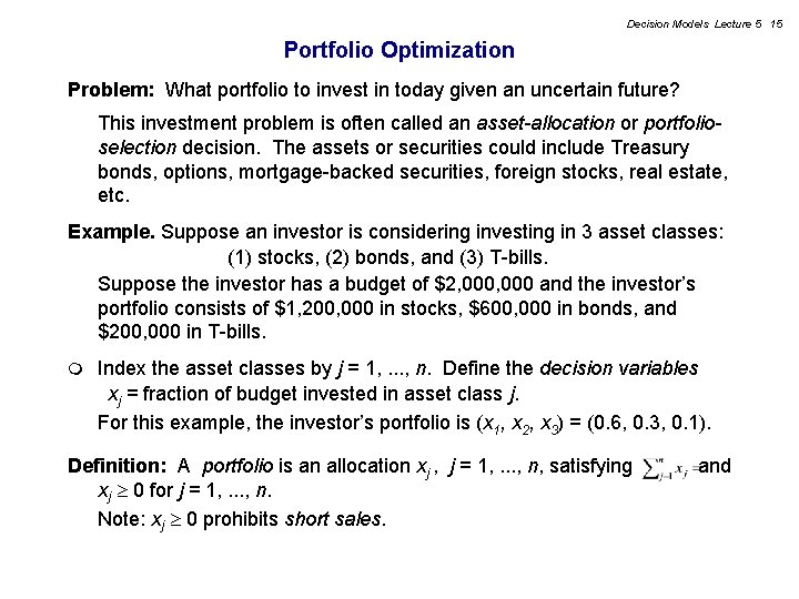
Decision Models Lecture 5 15 Portfolio Optimization Problem: What portfolio to invest in today given an uncertain future? This investment problem is often called an asset-allocation or portfolioselection decision. The assets or securities could include Treasury bonds, options, mortgage-backed securities, foreign stocks, real estate, etc. Example. Suppose an investor is considering investing in 3 asset classes: (1) stocks, (2) bonds, and (3) T-bills. Suppose the investor has a budget of $2, 000 and the investor’s portfolio consists of $1, 200, 000 in stocks, $600, 000 in bonds, and $200, 000 in T-bills. m Index the asset classes by j = 1, . . . , n. Define the decision variables xj = fraction of budget invested in asset class j. For this example, the investor’s portfolio is (x 1, x 2, x 3) = (0. 6, 0. 3, 0. 1). Definition: A portfolio is an allocation xj , j = 1, . . . , n, satisfying xj 0 for j = 1, . . . , n. Note: xj 0 prohibits short sales. and

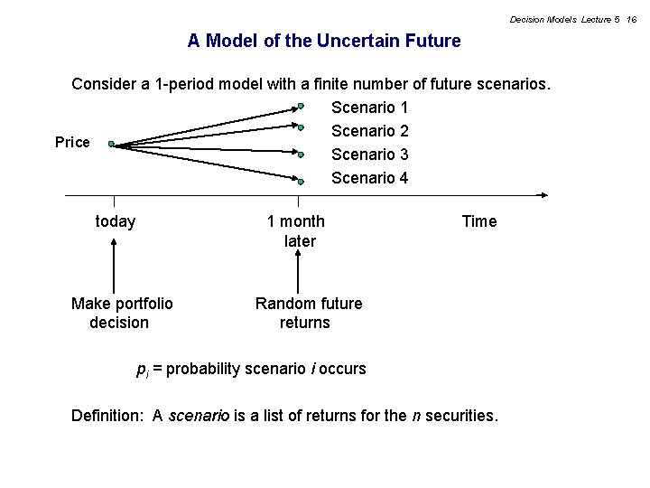
Decision Models Lecture 5 16 A Model of the Uncertain Future Consider a 1 -period model with a finite number of future scenarios. Scenario 1 Scenario 2 Price Scenario 3 Scenario 4 today 1 month later Make portfolio decision Time Random future returns pi = probability scenario i occurs Definition: A scenario is a list of returns for the n securities.

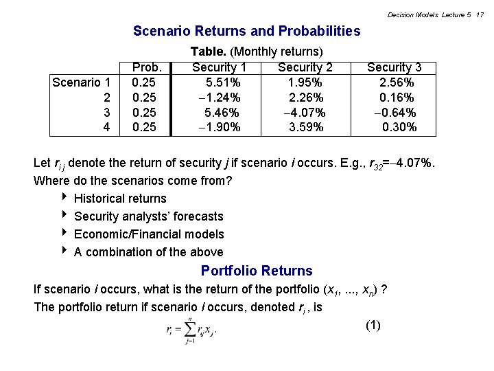
Decision Models Lecture 5 17 Scenario Returns and Probabilities Scenario 1 2 3 4 Prob. 0. 25 Table. (Monthly returns) Security 1 Security 2 5. 51% 1. 95% 1. 24% 2. 26% 5. 46% 4. 07% 1. 90% 3. 59% Security 3 2. 56% 0. 16% 0. 64% 0. 30% Let ri j denote the return of security j if scenario i occurs. E. g. , r 32= 4. 07%. Where do the scenarios come from? 4 Historical returns 4 Security analysts’ forecasts 4 Economic/Financial models 4 A combination of the above Portfolio Returns If scenario i occurs, what is the return of the portfolio (x 1, . . . , xn) ? The portfolio return if scenario i occurs, denoted ri , is (1)

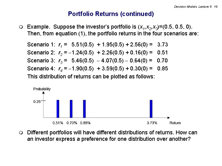
Decision Models Lecture 5 18 Portfolio Returns (continued) m Example. Suppose the investor’s portfolio is (x 1, x 2, x 3)=(0. 5, 0). Then, from equation (1), the portfolio returns in the four scenarios are: Scenario 1: r 1 = 5. 51(0. 5) + 1. 95(0. 5) + 2. 56(0) = Scenario 2: r 2 = 1. 24(0. 5) + 2. 26(0. 5) + 0. 16(0) = Scenario 3: r 3 = 5. 46(0. 5) 4. 07(0. 5) 0. 64(0) = Scenario 4: r 4 = 1. 90(0. 5) + 3. 59(0. 5) + 0. 30(0) = This distribution of returns can be plotted as follows: m 3. 73 0. 51 0. 70 0. 85 Different portfolios will have different distributions of returns. How can an investor express a preference for one distribution over another?

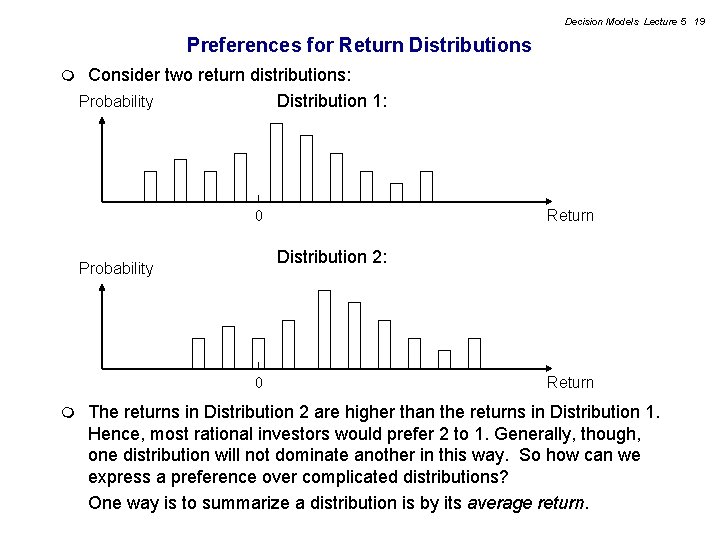
Decision Models Lecture 5 19 Preferences for Return Distributions m Consider two return distributions: Probability Distribution 1: Return 0 Distribution 2: Probability 0 m Return The returns in Distribution 2 are higher than the returns in Distribution 1. Hence, most rational investors would prefer 2 to 1. Generally, though, one distribution will not dominate another in this way. So how can we express a preference over complicated distributions? One way is to summarize a distribution is by its average return.

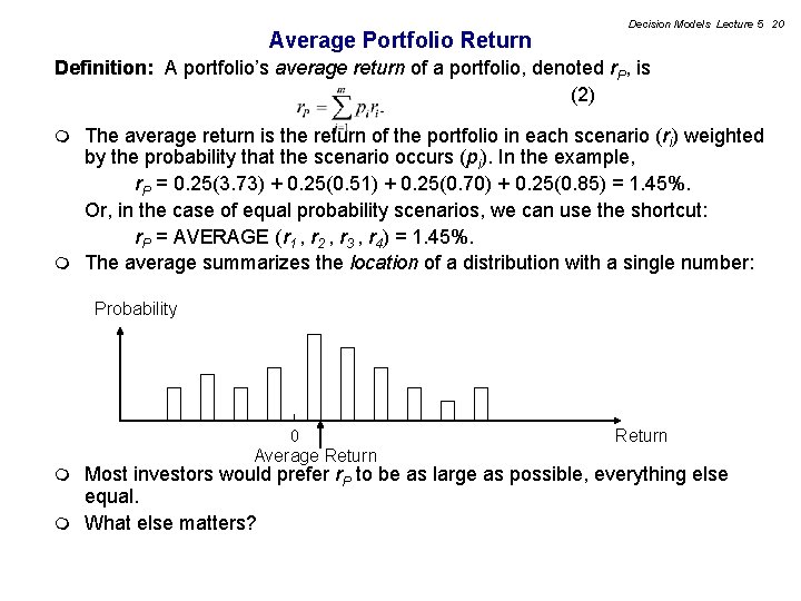
Average Portfolio Return Decision Models Lecture 5 20 Definition: A portfolio’s average return of a portfolio, denoted r. P, is (2) The average return is the return of the portfolio in each scenario (ri) weighted by the probability that the scenario occurs (pi). In the example, r. P = 0. 25(3. 73) + 0. 25(0. 51) + 0. 25(0. 70) + 0. 25(0. 85) = 1. 45%. Or, in the case of equal probability scenarios, we can use the shortcut: r. P = AVERAGE (r 1 , r 2 , r 3 , r 4) = 1. 45%. m The average summarizes the location of a distribution with a single number: m Probability 0 Average Return Most investors would prefer r. P to be as large as possible, everything else equal. m What else matters? m

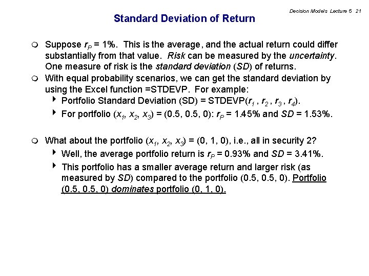
Standard Deviation of Return Decision Models Lecture 5 21 Suppose r. P = 1%. This is the average, and the actual return could differ substantially from that value. Risk can be measured by the uncertainty. One measure of risk is the standard deviation (SD) of returns. m With equal probability scenarios, we can get the standard deviation by using the Excel function =STDEVP. For example: 4 Portfolio Standard Deviation (SD) = STDEVP(r 1 , r 2 , r 3 , r 4). 4 For portfolio (x 1, x 2, x 3) = (0. 5, 0): r. P = 1. 45% and SD = 1. 53%. m m What about the portfolio (x 1, x 2, x 3) = (0, 1, 0), i. e. , all in security 2? 4 Well, the average portfolio return is r. P = 0. 93% and SD = 3. 41%. 4 This portfolio has a smaller average return and larger risk (as measured by SD) compared to the portfolio (0. 5, 0). Portfolio (0. 5, 0) dominates portfolio (0, 1, 0).

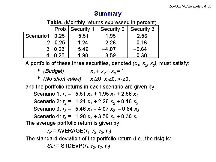
Decision Models Lecture 5 22 Summary Table. (Monthly returns expressed in percent) Prob. Security 1 Security 2 Security 3 Scenario 1 0. 25 5. 51 1. 95 2. 56 2 0. 25 1. 24 2. 26 0. 16 3 0. 25 5. 46 4. 07 0. 64 4 0. 25 1. 90 3. 59 0. 30 A portfolio of these three securities, denoted (x 1, x 2, x 3), must satisfy: 4 (Budget) x 1 + x 2 + x 3 = 1 4 (No short sales) x 1 0, x 2 0, x 3 0, and the portfolio returns in each scenario are given by: Scenario 1: r 1 = 5. 51 x 1 + 1. 95 x 2 + 2. 56 x 3 Scenario 2: r 2 = 1. 24 x 1 + 2. 26 x 2 + 0. 16 x 3 Scenario 3: r 3 = 5. 46 x 1 4. 07 x 2 0. 64 x 3 Scenario 4: r 4 = 1. 90 x 1 + 3. 59 x 2 + 0. 30 x 3 The average portfolio return is given by: r. P = AVERAGE(r 1, r 2, r 3, r 4) The standard deviation of the portfolio return (i. e. , the risk) is: SD = STDEVP(r 1, r 2, r 3, r 4)

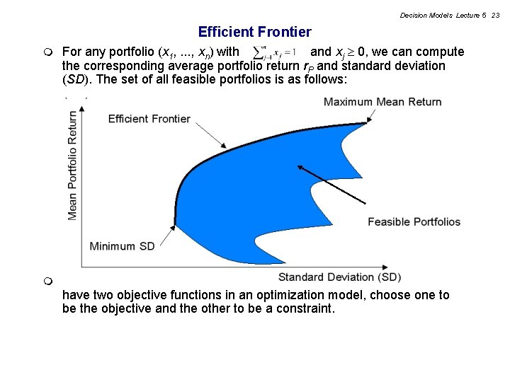
Decision Models Lecture 5 23 Efficient Frontier m For any portfolio (x 1, . . . , xn) with and xj 0, we can compute the corresponding average portfolio return r. P and standard deviation (SD). The set of all feasible portfolios is as follows: m Average return and risk are two conflicting objectives. Since we can’t have two objective functions in an optimization model, choose one to be the objective and the other to be a constraint.

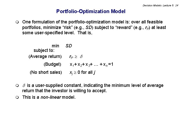
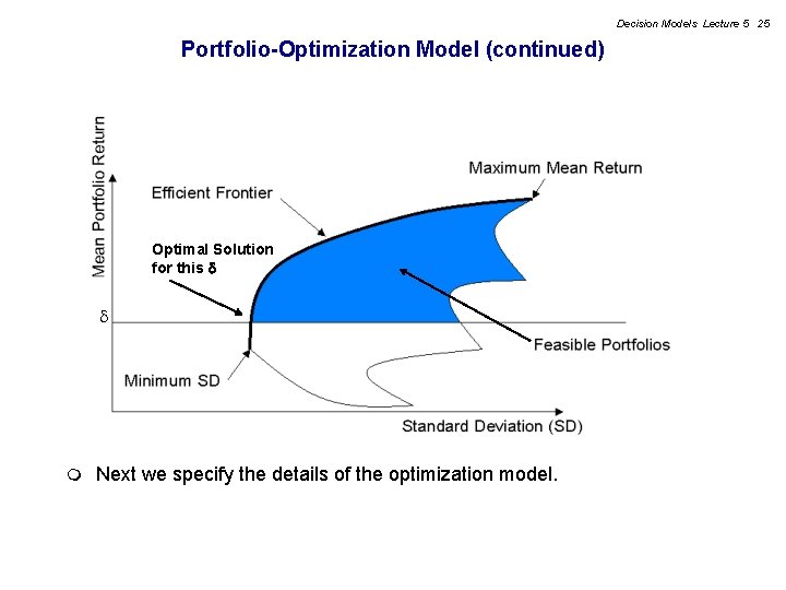
Decision Models Lecture 5 24 Portfolio-Optimization Model m One formulation of the portfolio-optimization model is: over all feasible portfolios, minimize “risk” (e. g. , SD) subject to “reward” (e. g. , r. P) at least some user-specified level. That is, min SD subject to: (Average return) r. P (Budget) (No short sales) m x 1+ x 2+ x 3+ … + xn =1 xj 0 for all j is a user-supplied constant, indicating the minimum level of average return that the investor is willing to accept. m This is a non-linear model.

Decision Models Lecture 5 25 Portfolio-Optimization Model (continued) Optimal Solution for this m Next we specify the details of the optimization model.

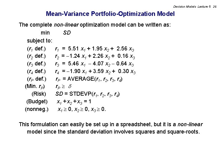
Decision Models Lecture 5 26 Mean-Variance Portfolio-Optimization Model The complete non-linear optimization model can be written as: min SD subject to: (r 1 def. ) r 1 = 5. 51 x 1 + 1. 95 x 2 + 2. 56 x 3 (r 2 def. ) r 2 = 1. 24 x 1 + 2. 26 x 2 + 0. 16 x 3 (r 3 def. ) r 3 = 5. 46 x 1 4. 07 x 2 0. 64 x 3 (r 4 def. ) r 4 = 1. 90 x 1 + 3. 59 x 2 + 0. 30 x 3 (r. P def. ) r. P = AVERAGE(r 1, r 2, r 3, r 4) (Min. r. P) r. P (Risk) SD = STDEVP(r 1, r 2, r 3, r 4) (Budget) x 1 + x 2 + x 3 = 1 (nonneg. ) x 1 0, x 2 0, x 3 0. This formulation can easily be set up in a spreadsheet, but it is a non-linear model since the standard deviation involves squares and square-roots.

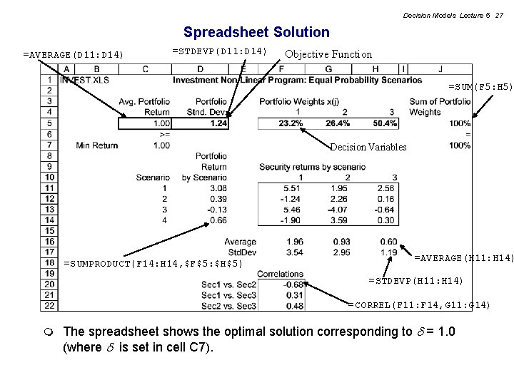
Decision Models Lecture 5 27 Spreadsheet Solution =AVERAGE(D 11: D 14) =STDEVP(D 11: D 14) Objective Function =SUM(F 5: H 5) Decision Variables =SUMPRODUCT(F 14: H 14, $F$5: $H$5) =AVERAGE(H 11: H 14) =STDEVP(H 11: H 14) =CORREL(F 11: F 14, G 11: G 14) m The spreadsheet shows the optimal solution corresponding to = 1. 0 (where is set in cell C 7).

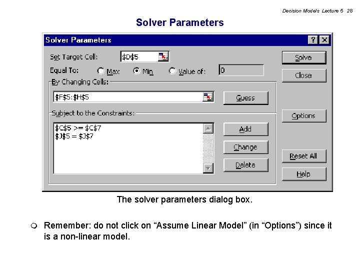
Decision Models Lecture 5 28 Solver Parameters The solver parameters dialog box. m Remember: do not click on “Assume Linear Model” (in “Options”) since it is a non-linear model.

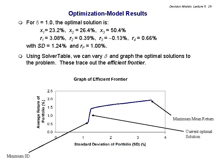
Decision Models Lecture 5 29 Optimization-Model Results m For = 1. 0, the optimal solution is: x 1= 23. 2%, x 2 = 26. 4%, x 3 = 50. 4% r 1 = 3. 08%, r 2 = 0. 39%, r 3 = 0. 13%, r 4 = 0. 66% with SD = 1. 24% and r. P = 1. 00%. m Using Solver. Table, we can vary and graph the optimal solutions to the problem. These trace out the efficient frontier. Maximum Mean Return Current optimal Solution Minimum SD

Decision Models Lecture 5 30 Comments on the Mean-Variance Model Alternate formulation: maximize return subject to a user-specified maximum risk (SD). m The mean-variance approach leads to a nonlinear model 4 This non-linear model is more difficult to solve than a linear one, but Excel can solve it. 4 Variance penalizes upside and downside returns 4 Less sensitivity-analysis information available with nonlinear programs 4 Right-hand side ranges are not given for nonlinear models m m Alternative models: Use a measure of risk, e. g. Average Downside Risk (ADR), which can be formulated as a linear model. See the readings book for details (“Portfolio Optimization Using Linear Programming”).

Decision Models Lecture 5 31 Comparison of Scenario Approach with Variance-Covariance Approach m An alternate method of formulating a mean-variance portfolio optimization model involves computing the variance-covariance matrix of the security returns. m Because the scenario approach uses the security returns directly, it does not require computation of the variance-covariance matrix. m The two approaches give the same answer! (They are really identical. ) m Since the scenario-based model uses the data directly, the historical correlations between security returns are used implicitly, and need not be computed.

Decision Models Lecture 5 32 Summary Integer Programming - A Plant Location Example m Portfolio Optimization 4 Modeling uncertainty with scenarios 4 Definitions of reward and risk 4 Tradeoff between two conflicting objectives 4 The Efficient Frontier 4 Setting up the Model 4 Solving the Model 4 Looking at the Results m For next class m Optional readings: “Exploring the New Efficient Frontier” and “Asset Allocation in a Downside-Risk Framework” in the readings book.