Decision List LING 572 Fei Xia 11206 Outline

Decision List LING 572 Fei Xia 1/12/06

Outline • Basic concepts and properties • Case study

Definitions • A decision list (DL) is an ordered list of conjunctive rules. – Rules can overlap, so the order is important. • A k-DL: the length of every rule is at most k. • A decision tree determines an example’s class by using the first matched rule.

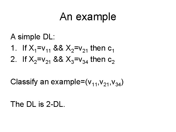
An example A simple DL: 1. If X 1=v 11 && X 2=v 21 then c 1 2. If X 2=v 21 && X 3=v 34 then c 2 Classify an example=(v 11, v 21, v 34) The DL is 2 -DL.

Rivest’s paper • It assumes that all attributes (including goal attribute) are binary. • It shows DL is easily learnable from examples.

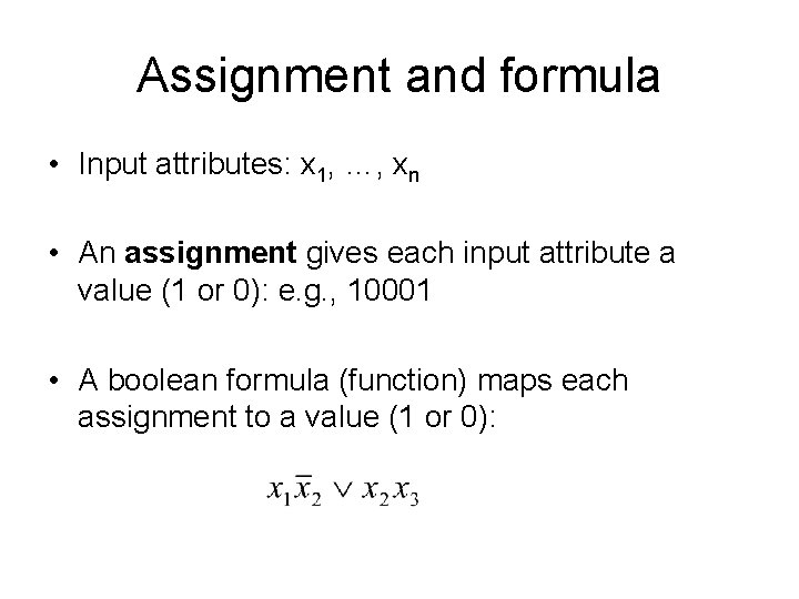
Assignment and formula • Input attributes: x 1, …, xn • An assignment gives each input attribute a value (1 or 0): e. g. , 10001 • A boolean formula (function) maps each assignment to a value (1 or 0):

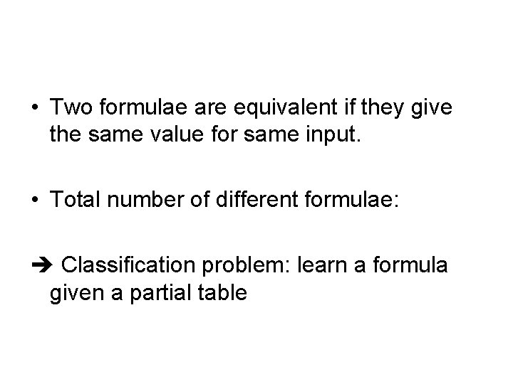
• Two formulae are equivalent if they give the same value for same input. • Total number of different formulae: Classification problem: learn a formula given a partial table

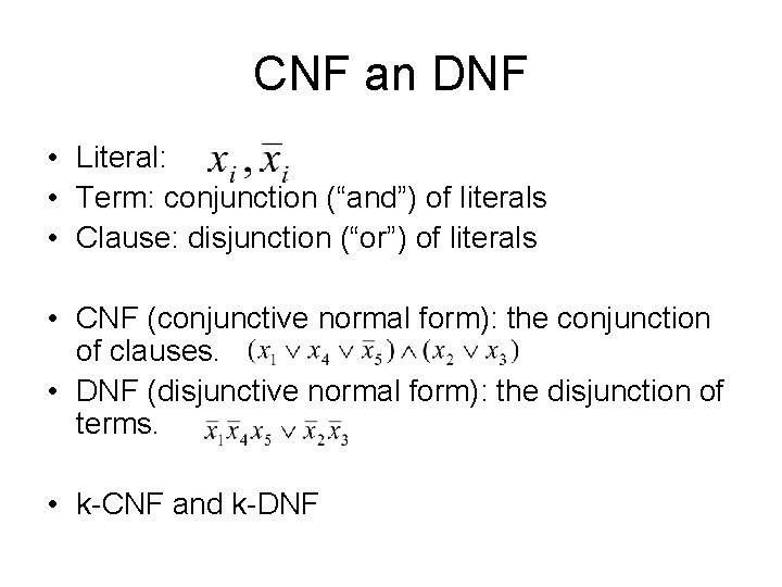
CNF an DNF • Literal: • Term: conjunction (“and”) of literals • Clause: disjunction (“or”) of literals • CNF (conjunctive normal form): the conjunction of clauses. • DNF (disjunctive normal form): the disjunction of terms. • k-CNF and k-DNF

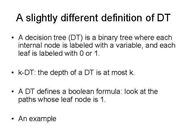
A slightly different definition of DT • A decision tree (DT) is a binary tree where each internal node is labeled with a variable, and each leaf is labeled with 0 or 1. • k-DT: the depth of a DT is at most k. • A DT defines a boolean formula: look at the paths whose leaf node is 1. • An example

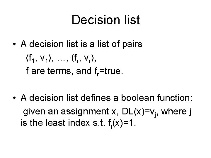
Decision list • A decision list is a list of pairs (f 1, v 1), …, (fr, vr), fi are terms, and fr=true. • A decision list defines a boolean function: given an assignment x, DL(x)=vj, where j is the least index s. t. fj(x)=1.

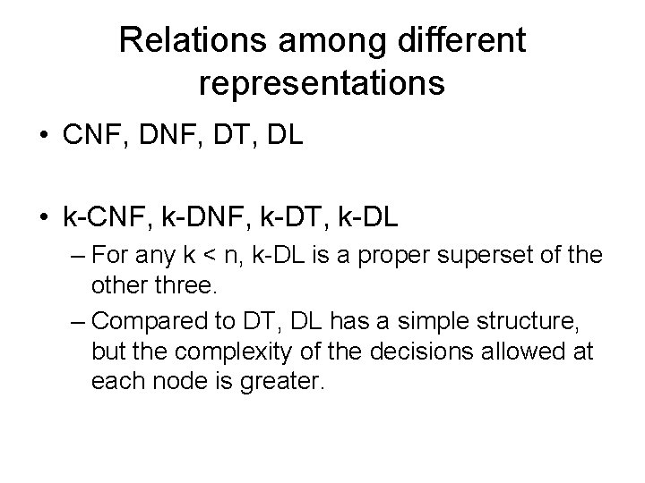
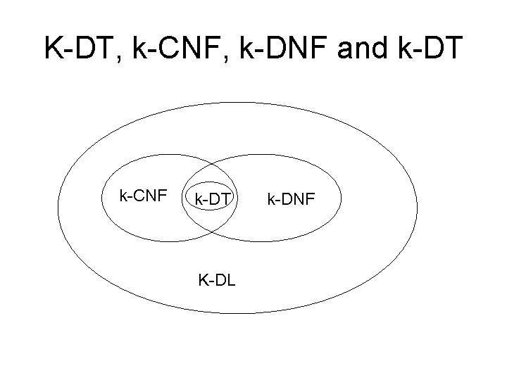
Relations among different representations • CNF, DT, DL • k-CNF, k-DT, k-DL – For any k < n, k-DL is a proper superset of the other three. – Compared to DT, DL has a simple structure, but the complexity of the decisions allowed at each node is greater.

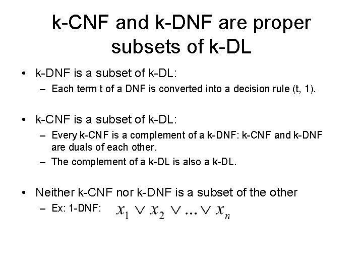
k-CNF and k-DNF are proper subsets of k-DL • k-DNF is a subset of k-DL: – Each term t of a DNF is converted into a decision rule (t, 1). • k-CNF is a subset of k-DL: – Every k-CNF is a complement of a k-DNF: k-CNF and k-DNF are duals of each other. – The complement of a k-DL is also a k-DL. • Neither k-CNF nor k-DNF is a subset of the other – Ex: 1 -DNF:

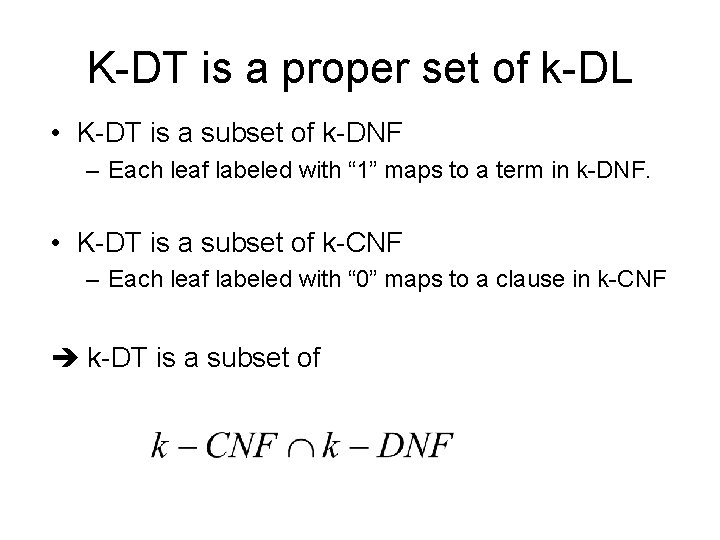
K-DT is a proper set of k-DL • K-DT is a subset of k-DNF – Each leaf labeled with “ 1” maps to a term in k-DNF. • K-DT is a subset of k-CNF – Each leaf labeled with “ 0” maps to a clause in k-CNF k-DT is a subset of

K-DT, k-CNF, k-DNF and k-DT k-CNF k-DT K-DL k-DNF

Learnability • Positive examples vs. negative examples of the concept being learned. – In some domains, positive examples are easier to collect. • A sample is a set of examples. • A boolean function is consistent with a sample if it does not contradict any example in the sample.

Two properties of a learning algorithm • A learning algorithm is economical if it requires few examples to identify the correct concept. • A learning algorithm is efficient if it requires little computational effort to identify the correct concept. We prefer algorithms that are both economical and efficient.

Hypothesis space • Hypothesis space F: a set of concepts that are being considered. • Hopefully, the concept being learned should be in the hypothesis space of a learning algorithm. • The goal of a learning algorithm is to select the right concept from F given the training data.

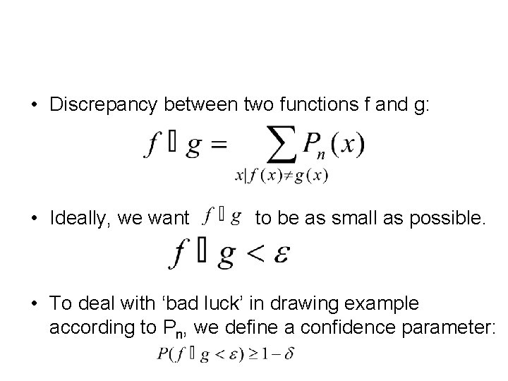
• Discrepancy between two functions f and g: • Ideally, we want to be as small as possible. • To deal with ‘bad luck’ in drawing example according to Pn, we define a confidence parameter:

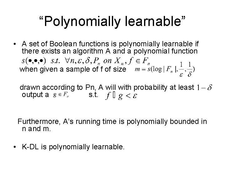
“Polynomially learnable” • A set of Boolean functions is polynomially learnable if there exists an algorithm A and a polynomial function when given a sample of f of size drawn according to Pn, A will with probability at least output a s. t. Furthermore, A’s running time is polynomially bounded in n and m. • K-DL is polynomially learnable.

How to build a decision list • Decision tree Decision list • Greedy, iterative algorithm that builds DLs directly.

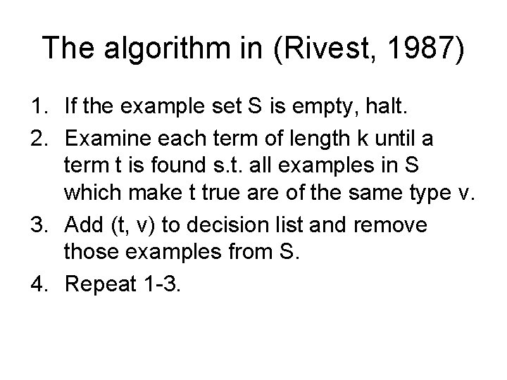
The algorithm in (Rivest, 1987) 1. If the example set S is empty, halt. 2. Examine each term of length k until a term t is found s. t. all examples in S which make t true are of the same type v. 3. Add (t, v) to decision list and remove those examples from S. 4. Repeat 1 -3.

The general greedy algorithm • Rule. List=[], E=training_data • Repeat until E is empty or gain is small – f = Find_best_feature(E) – Let E’ be the examples covered by f – Let c be the most common class in E’ – Add (f, c) to Rule. List – E=E – E’

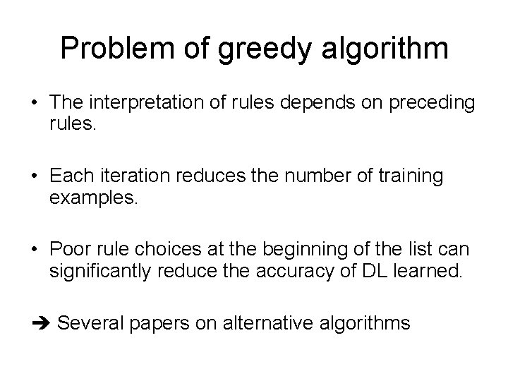
Problem of greedy algorithm • The interpretation of rules depends on preceding rules. • Each iteration reduces the number of training examples. • Poor rule choices at the beginning of the list can significantly reduce the accuracy of DL learned. Several papers on alternative algorithms

Summary of (Rivest, 1987) • Formal definition of DL • Show the relation between k-DL, k-CNF, k. DNF and k-DL. • Prove that k-DL is polynomially learnable. • Give a simple greedy algorithm to build k. DL.

Outline • Basic concepts and properties • Case study

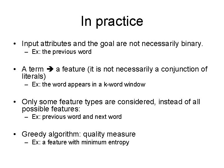
In practice • Input attributes and the goal are not necessarily binary. – Ex: the previous word • A term a feature (it is not necessarily a conjunction of literals) – Ex: the word appears in a k-word window • Only some feature types are considered, instead of all possible features: – Ex: previous word and next word • Greedy algorithm: quality measure – Ex: a feature with minimum entropy

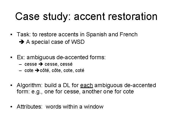
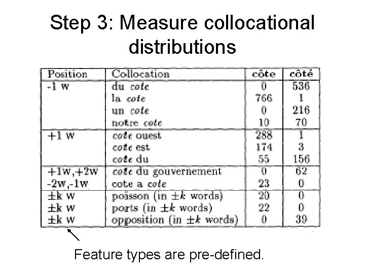
Case study: accent restoration • Task: to restore accents in Spanish and French A special case of WSD • Ex: ambiguous de-accented forms: – cesse, cessé – cote côté, côte, coté • Algorithm: build a DL for each ambiguous de-accented form: e. g. , one for cesse, another one for cote • Attributes: words within a window

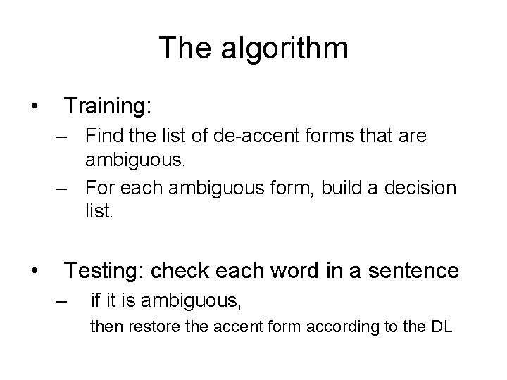
The algorithm • Training: – Find the list of de-accent forms that are ambiguous. – For each ambiguous form, build a decision list. • Testing: check each word in a sentence – if it is ambiguous, then restore the accent form according to the DL

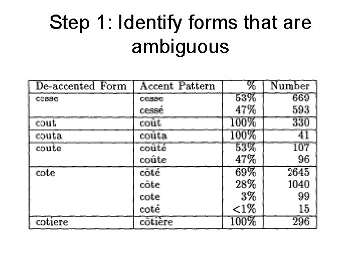
Step 1: Identify forms that are ambiguous

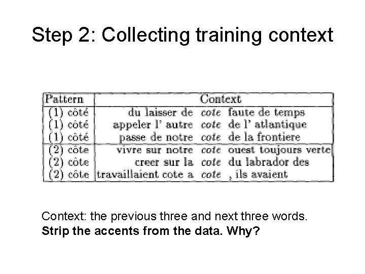
Step 2: Collecting training context Context: the previous three and next three words. Strip the accents from the data. Why?

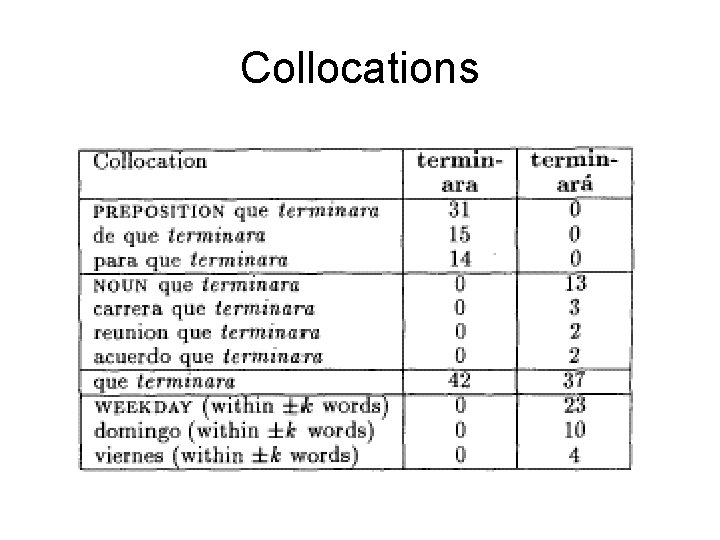
Step 3: Measure collocational distributions Feature types are pre-defined.

Collocations

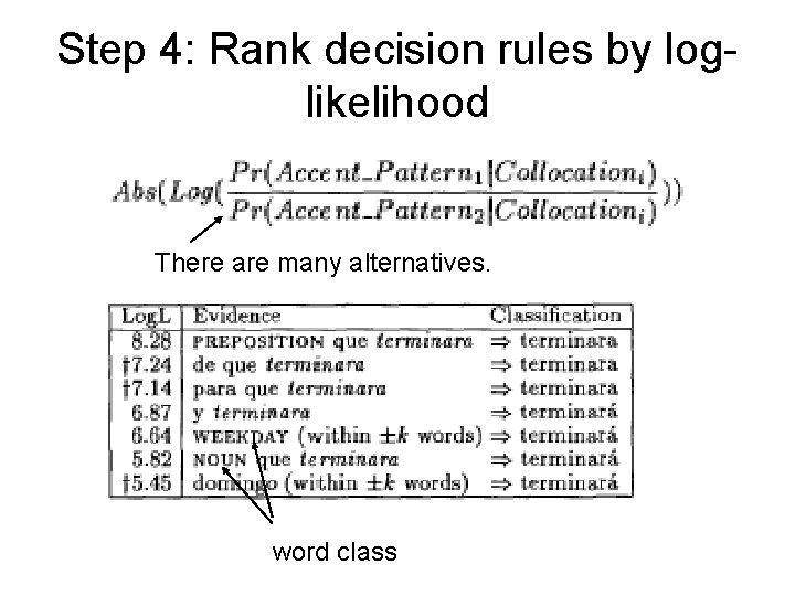
Step 4: Rank decision rules by loglikelihood There are many alternatives. word class

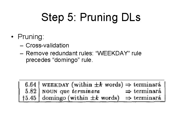
Step 5: Pruning DLs • Pruning: – Cross-validation – Remove redundant rules: “WEEKDAY” rule precedes “domingo” rule.

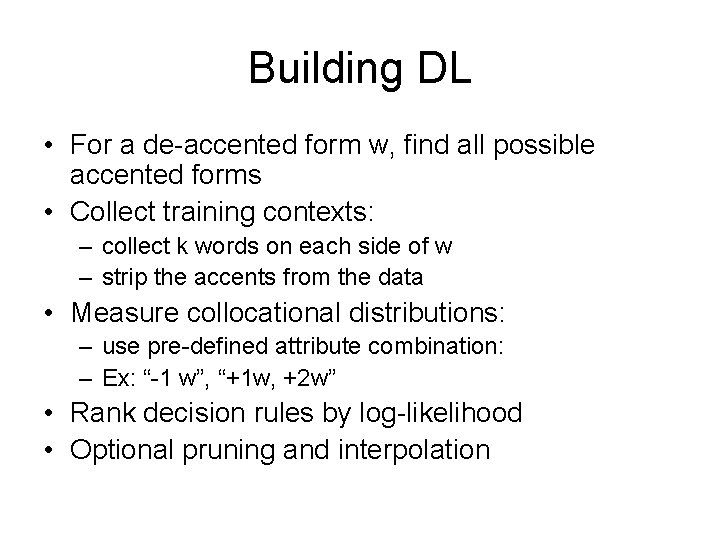
Building DL • For a de-accented form w, find all possible accented forms • Collect training contexts: – collect k words on each side of w – strip the accents from the data • Measure collocational distributions: – use pre-defined attribute combination: – Ex: “-1 w”, “+1 w, +2 w” • Rank decision rules by log-likelihood • Optional pruning and interpolation

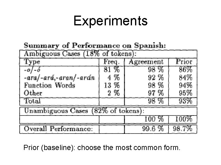
Experiments Prior (baseline): choose the most common form.

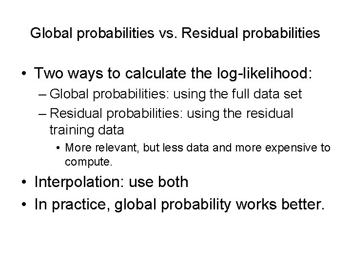
Global probabilities vs. Residual probabilities • Two ways to calculate the log-likelihood: – Global probabilities: using the full data set – Residual probabilities: using the residual training data • More relevant, but less data and more expensive to compute. • Interpolation: use both • In practice, global probability works better.

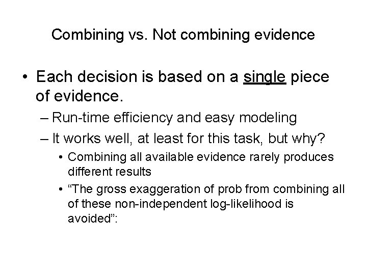
Combining vs. Not combining evidence • Each decision is based on a single piece of evidence. – Run-time efficiency and easy modeling – It works well, at least for this task, but why? • Combining all available evidence rarely produces different results • “The gross exaggeration of prob from combining all of these non-independent log-likelihood is avoided”:

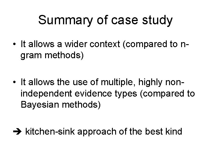
Summary of case study • It allows a wider context (compared to ngram methods) • It allows the use of multiple, highly nonindependent evidence types (compared to Bayesian methods) kitchen-sink approach of the best kind

Advance topics

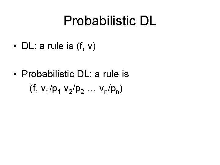
Probabilistic DL • DL: a rule is (f, v) • Probabilistic DL: a rule is (f, v 1/p 1 v 2/p 2 … vn/pn)

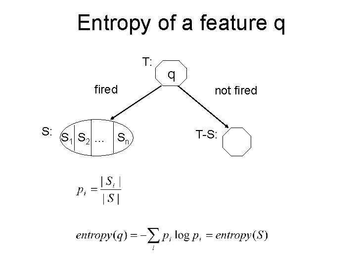
Entropy of a feature q T: fired S: S S 1 2 … Sn q not fired T-S:

Algorithms for building DL • • • AQ algorithm (Michalski, 1969) CN 2 algorithm (Clark and Niblett, 1989) Segal and Etzioni (1994) Goodman (2002) …

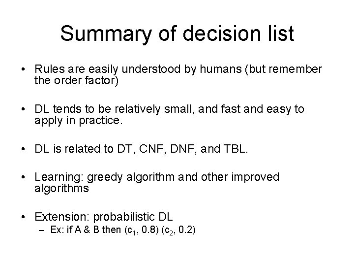
Summary of decision list • Rules are easily understood by humans (but remember the order factor) • DL tends to be relatively small, and fast and easy to apply in practice. • DL is related to DT, CNF, DNF, and TBL. • Learning: greedy algorithm and other improved algorithms • Extension: probabilistic DL – Ex: if A & B then (c 1, 0. 8) (c 2, 0. 2)