Debugging Schema Mappings with Routes Laura Chiticariu UC

Debugging Schema Mappings with Routes Laura Chiticariu UC Santa Cruz (joint work with Wang-Chiew Tan) 1

SPIDER: A Schema Mapping Debugger Demo group B Today 14: 00 -15: 30 Thursday 11: 00 -12: 30 2

Schema Mappings p A schema mapping is a logical assertion that describes the correspondence between two schemas n p Key element in data exchange and data integration systems Data Exchange [FKMP 05] n Translate data conforming to a source schema S into data conforming to a target schema T so that the schema mapping M is satisfied M Schema S I Source instance Schema T J Target instance 3

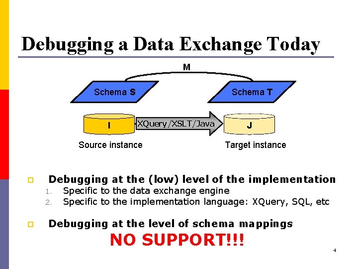
Debugging a Data Exchange Today M Schema S I Schema T XQuery/XSLT/Java Source instance p Target instance Debugging at the (low) level of the implementation 1. 2. p J Specific to the data exchange engine Specific to the implementation language: XQuery, SQL, etc Debugging at the level of schema mappings NO SUPPORT!!! 4

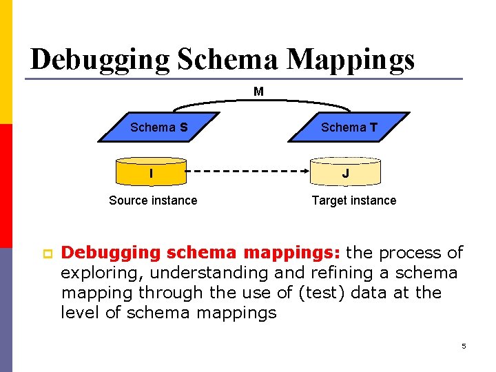
Debugging Schema Mappings M Schema S I Source instance p Schema T J Target instance Debugging schema mappings: the process of exploring, understanding and refining a schema mapping through the use of (test) data at the level of schema mappings 5

Outline p Overview p Motivation p Debugging schema mappings with routes n n Motivating example What are routes? Computing routes Related work p Performance evaluation p Conclusions 6

Motivation p Schema mappings are good n n p Hide implementation details, allow for optimization Typically easier to understand vs. SQL/XSLT/XQuery/Java Serve a similar goal as model management [Bernstein 03, MBHR 05] Uniformity in specifying and debugging n p Higher-level, declarative programming constructs Reduce programming effort by allowing a user to specify and debug at the level of schema mappings Schema mappings are often generated by schema matching tools n n Close to user’s intention, but may need further refinements Hard to understand without the help of tools 7

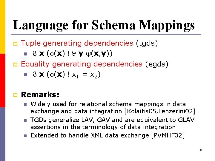
Language for Schema Mappings p p p Tuple generating dependencies (tgds) n 8 x ( (x) ! 9 y (x, y)) Equality generating dependencies (egds) n 8 x ( (x) ! x 1 = x 2) Remarks: n n n Widely used for relational schema mappings in data exchange and data integration [Kolaitis 05, Lenzerini 02] TGDs generalize LAV, GAV and are equivalent to GLAV assertions in the terminology of data integration Extended to handle XML data exchange [PVMHF 02] 8

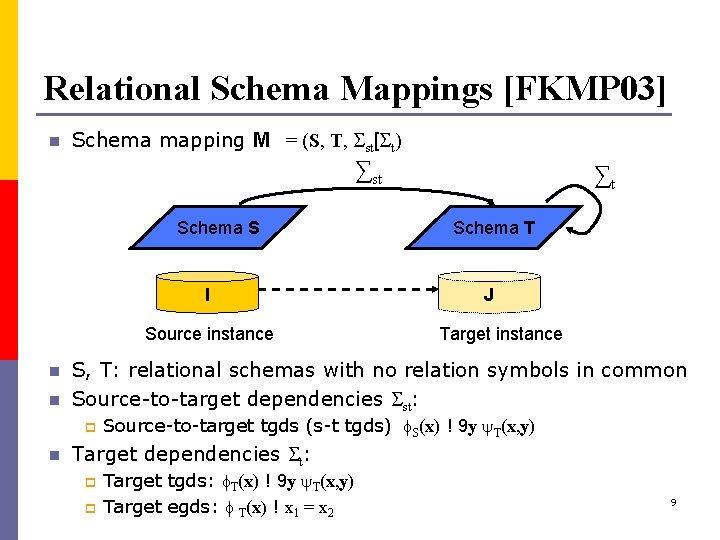
Relational Schema Mappings [FKMP 03] n Schema mapping M = (S, T, st[ t) ∑st Schema S I Source instance n n Schema T J Target instance S, T: relational schemas with no relation symbols in common Source-to-target dependencies st: p n ∑t Source-to-target tgds (s-t tgds) S(x) ! 9 y T(x, y) Target dependencies t: p p Target tgds: T(x) ! 9 y T(x, y) Target egds: T(x) ! x 1 = x 2 9

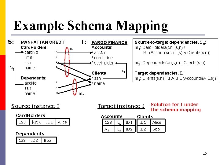
Example Schema Mapping S: fk 1 MANHATTAN CREDIT Card. Holders: m 1 card. No ² limit ² ssn ² name ² Dependents: acc. No ssn name ² ² ² ID 1 ID 2 m 2: Dependents(an, s, n) ! Clients(s, n) Target dependencies, t: m 3: Clients(s, n) ! A L (Accounts(A, L, s)) Target instance J Accounts Dependents 123 m 3 Source-to-target dependencies, st: m 1: Card. Holders(cn, l, s, n) ! 9 L (Accounts(cn, L, s) Clients(s, n)) m 2 Card. Holders $15 K FARGO FINANCE Accounts: ² acc. No ² credit. Line ² acc. Holder Clients: ² ssn ² name Source instance I 123 T: Alice Solution for I under the schema mapping Clients 123 L 1 ID 1 Alice A 2 L 2 ID 2 Bob 10

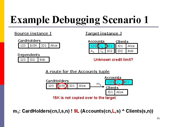
Example Debugging Scenario 1 Target instance J Source instance I Card. Holders 123 $15 K Accounts ID 1 Alice Dependents 123 ID 2 Clients 123 L 1 ID 1 Alice A 2 L 2 ID 2 Bob Unknown credit limit? Bob A route for the Accounts tuple Accounts Card. Holders 123 $15 K ID 1 Alice m 1 123 L 1 ID 1 Clients ID 1 Alice 15 K is not copied over to the target m 1: Card. Holders(cn, l, s, n) ! 9 L (Accounts(cn, L, s) ^ Clients(s, n)) 11

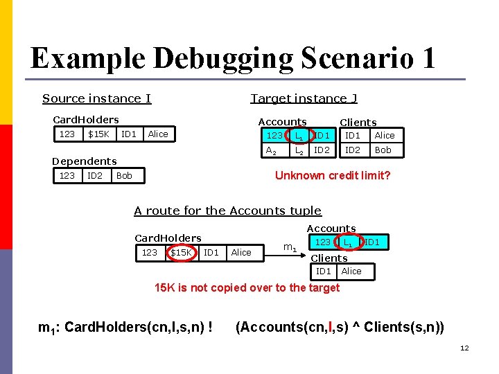
Example Debugging Scenario 1 Target instance J Source instance I Card. Holders 123 $15 K Accounts ID 1 Alice Dependents 123 ID 2 Clients 123 L 1 ID 1 Alice A 2 L 2 ID 2 Bob Unknown credit limit? Bob A route for the Accounts tuple Accounts Card. Holders 123 $15 K ID 1 Alice m 1 123 L 1 ID 1 Clients ID 1 Alice 15 K is not copied over to the target m 1: Card. Holders(cn, l, s, n) ! (Accounts(cn, l, s) ^ Clients(s, n)) 12

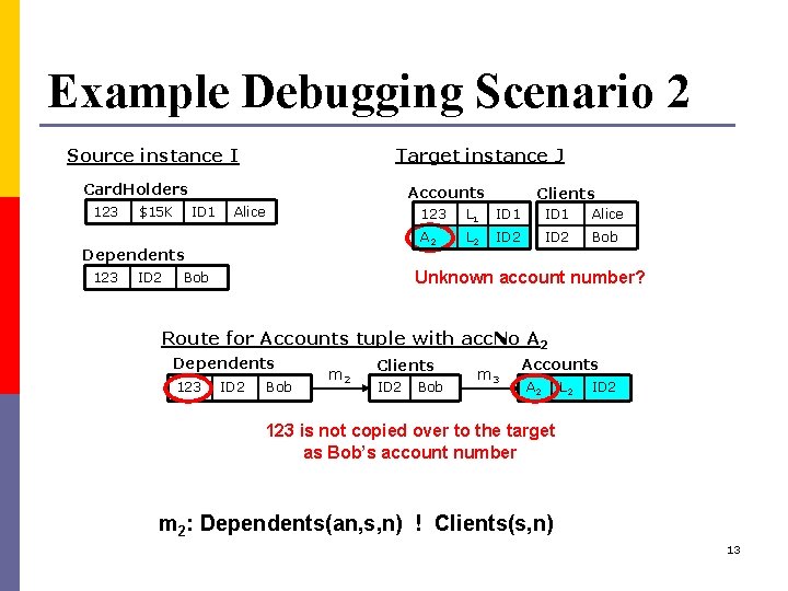
Example Debugging Scenario 2 Target instance J Source instance I Card. Holders 123 $15 K Accounts ID 1 Alice Dependents 123 ID 2 Clients 123 L 1 ID 1 Alice A 2 L 2 ID 2 Bob Unknown account number? Bob Route for Accounts tuple with acc. No A 2 Dependents 123 ID 2 Bob m 2 Clients ID 2 Bob m 3 Accounts A 2 L 2 ID 2 123 is not copied over to the target as Bob’s account number m 2: Dependents(an, s, n) ! Clients(s, n) 13

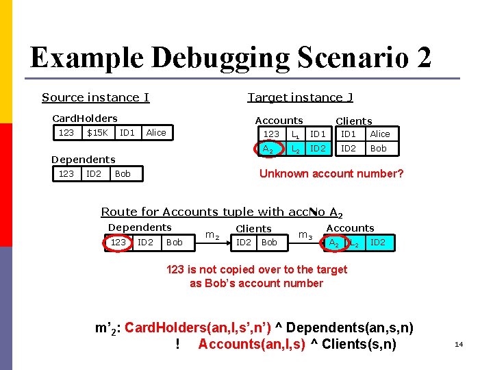
Example Debugging Scenario 2 Target instance J Source instance I Card. Holders 123 $15 K Accounts ID 1 Alice Dependents 123 ID 2 Clients 123 L 1 ID 1 Alice A 2 L 2 ID 2 Bob Unknown account number? Bob Route for Accounts tuple with acc. No A 2 Dependents 123 ID 2 Bob m 2 Clients ID 2 Bob m 3 Accounts A 2 L 2 ID 2 123 is not copied over to the target as Bob’s account number m’ 2: Card. Holders(an, l, s’, n’) ^ Dependents(an, s, n) ! Accounts(an, l, s) ^ Clients(s, n) 14

Debugging Schema Mappings with Routes p Main intuition: routes describe the relationships between source and target data with the schema mapping p Definition: Let: n n n M be a schema mapping I be a source instance J be a solution for I under M and Js µ J A route for Js with M and (I, J) is a finite non-empty sequence of satisfaction steps (I, ; ) m 1 , h 1 ! (I, J 1) mn , h n m 2 , h 2 ! … such that: n Ji µ J, mi 2 st [ t, where 1· i· n n Js µ Jn ! (I, Jn) 15

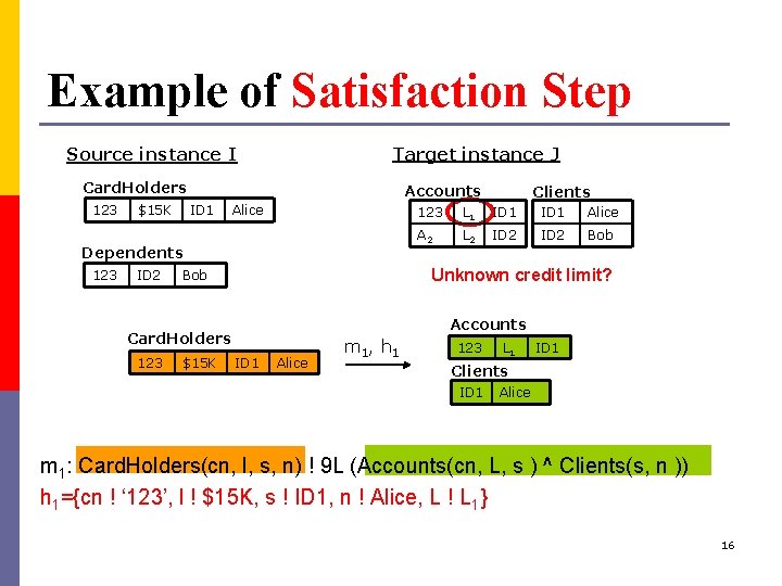
Example of Satisfaction Step Target instance J Source instance I Card. Holders 123 $15 K Accounts ID 1 Alice Dependents 123 ID 2 $15 K 123 L 1 ID 1 Alice A 2 L 2 ID 2 Bob Unknown credit limit? Bob Accounts Card. Holders 123 Clients ID 1 Alice m 1 , h 1 123 L 1 ID 1 Clients ID 1 Alice m 1: Card. Holders(cn, l, s, n) ! 9 L (Accounts(cn, L, s ) ^ Clients(s, n )) h 1={cn ! ‘ 123’, l ! $15 K, s ! ID 1, n ! Alice, L ! L 1} 16

Compute all routes p The schema mapping M is fixed p Input: source instance I, a solution J for I under M, a set of target tuples Js µ J Output: a forest representing all routes for Js p p Algorithm idea: n For each tuple t in Js, consider every possible 2 st [ t and h for witnessing t n Do the same for all target tuples encountered during the process until tuples from the source instance are obtained 17

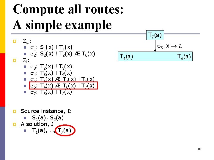
Compute all routes: A simple example p p st: n 1: n 2: t: n 3: n 4: n 5: n 6: n 7: S 1(x) ! T 1(x) S 2(x) ! T 2(x) Æ T 6(x) T 2(x) T 3(x) T 4(x) T 5(x) T 7(a) 6 , x a T 4(a) T 6(a) ! T 3(x) ! T 4(x) Æ T 1(x) ! T 5(x) Æ T 6(x) ! T 7(x) ! T 3(x) Source instance, I: n S 1(a), S 2(a) A solution, J: n T 1(a), …, T 7(a) 18

Compute all routes: A simple example p p st: n 1: n 2: t: n 3: n 4: n 5: n 6: n 7: S 1(x) ! T 1(x) S 2(x) ! T 2(x) Æ T 6(x) T 2(x) T 3(x) T 4(x) T 5(x) ! T 3(x) ! T 4(x) Æ T 1(x) ! T 5(x) Æ T 6(x) ! T 7(x) ! T 3(x) T 7(a) 6 T 4(a) T 6(a) 4 , x a T 3(a) Source instance, I: n S 1(a), S 2(a) A solution, J: n T 1(a), …, T 7(a) 19

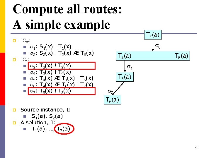
Compute all routes: A simple example p p st: n 1: n 2: t: n 3: n 4: n 5: n 6: n 7: S 1(x) ! T 1(x) S 2(x) ! T 2(x) Æ T 6(x) T 2(x) T 3(x) T 4(x) T 5(x) ! T 3(x) ! T 4(x) Æ T 1(x) ! T 5(x) Æ T 6(x) ! T 7(x) ! T 3(x) T 7(a) 6 T 4(a) T 6(a) 4 T 3(a) 7 T 5(a) Source instance, I: n S 1(a), S 2(a) A solution, J: n T 1(a), …, T 7(a) 20

Compute all routes: A simple example p p st: n 1: n 2: t: n 3: n 4: n 5: n 6: n 7: 6 S 1(x) ! T 1(x) S 2(x) ! T 2(x) Æ T 6(x) T 2(x) T 3(x) T 4(x) T 5(x) ! T 3(x) ! T 4(x) Æ T 1(x) ! T 5(x) Æ T 6(x) ! T 7(x) ! T 3(x) Source instance, I: n S 1(a), S 2(a) A solution, J: n T 1(a), …, T 7(a) T 4(a) T 6(a) 4 T 3(a) 7 T 5(a) 5 T 4(a) T 1(a) 1 S 1(a) 21

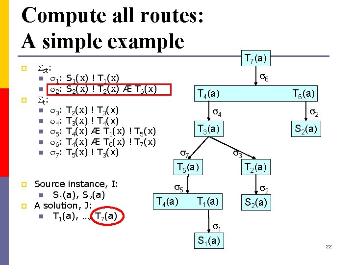
Compute all routes: A simple example p p st: n 1: n 2: t: n 3: n 4: n 5: n 6: n 7: 6 S 1(x) ! T 1(x) S 2(x) ! T 2(x) Æ T 6(x) T 2(x) T 3(x) T 4(x) T 5(x) ! T 3(x) ! T 4(x) Æ T 1(x) ! T 5(x) Æ T 6(x) ! T 7(x) ! T 3(x) Source instance, I: n S 1(a), S 2(a) A solution, J: n T 1(a), …, T 7(a) T 4(a) 4 2 T 3(a) S 2(a) 7 T 5(a) 5 T 4(a) T 6(a) T 1(a) 1 S 1(a) 3 T 2(a) 2 S 2(a) 22

Compute all routes: A simple example p p st: n 1: n 2: t: n 3: n 4: n 5: n 6: n 7: 6 S 1(x) ! T 1(x) S 2(x) ! T 2(x) Æ T 6(x) T 2(x) T 3(x) T 4(x) T 5(x) ! T 3(x) ! T 4(x) Æ T 1(x) ! T 5(x) Æ T 6(x) ! T 7(x) ! T 3(x) Source instance, I: n S 1(a), S 2(a) A solution, J: n T 1(a), …, T 7(a) T 4(a) T 6(a) 4 8 T 3(a) S 2(a) 7 T 5(a) 5 T 4(a) Route for T 7(a): 2, 3, 4, 8, 6 T 7(a) T 1(a) 1 S 1(a) 3 T 2(a) 2 S 2(a) 23

Properties of compute all routes p Completeness: Let F denote the route forest by our algorithm returned on Js. If R is a minimal route for Js, then it is represented in F. p Running time: polynomial in the sizes of I, J and Js n n p Every “branch of a tuple” once explored, is never explored again Polynomial number of branches for each tuple since M is fixed Challenge: n Exponentially many routes, but polynomial-size representation constructed in polynomial time 24

Compute one route p p p Our experimental results indicate that compute all routes can be expensive Generate one route fast and alternative routes as needed? Our solution: adapt compute all routes to compute only one route n Non-exhaustive: Stops when one witness is found. A witness that uses source tuples is preferred n Inference procedure: to deduce all consequences of a proven tuple and avoid recomputation of “branches” p n Key step for polynomial time analysis Completeness: If there is a route for Js, then our algorithm will produce a route for Js 25

Related work p Commercial data exchange systems n n e. g. , Altova Map. Force, Stylus Studio Use “lower-level” languages (e. g. , XSLT, XQuery) to specify the exchange p p p Debugging is done at this low level Source tuple centric Data viewer [YMHF 01] n Constructs an “example” source instance illustrative for the behavior of the schema mapping p n Complementary to our approach Works only for relational schema mappings 26

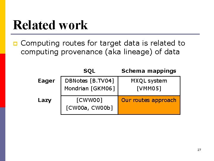
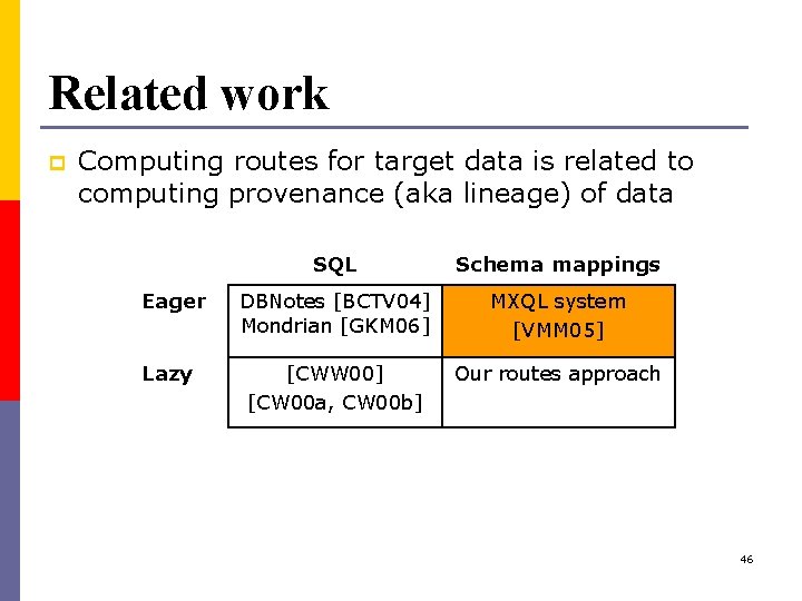
Related work p Computing routes for target data is related to computing provenance (aka lineage) of data Eager Lazy SQL Schema mappings DBNotes [B. TV 04] Mondrian [GKM 06] MXQL system [VMM 05] [CWW 00] [CW 00 a, CW 00 b] Our routes approach 27

Empirical Evaluation p Implementation: on top of the Clio data exchange system from IBM Almaden Research Center n n p Testbed: n n p Scalable: push computation to the database Handles relational and XML schema mappings [PVMHF 02] Created relational and XML schema mappings based on the TPCH schema Created schema mappings based on Mondial, DBLP and Amalgam schemas Methodology - measured the influence of: n n The sizes of I, J and Js The complexity of st [ t p i. e. , the number of tgds and the number of atoms in each tgd p Setup: P 4 2. 8 GHz, 2 Gb RAM, 256 MB DB 2 buffer pool p Our regret: No benchmark to base our comparisons 28

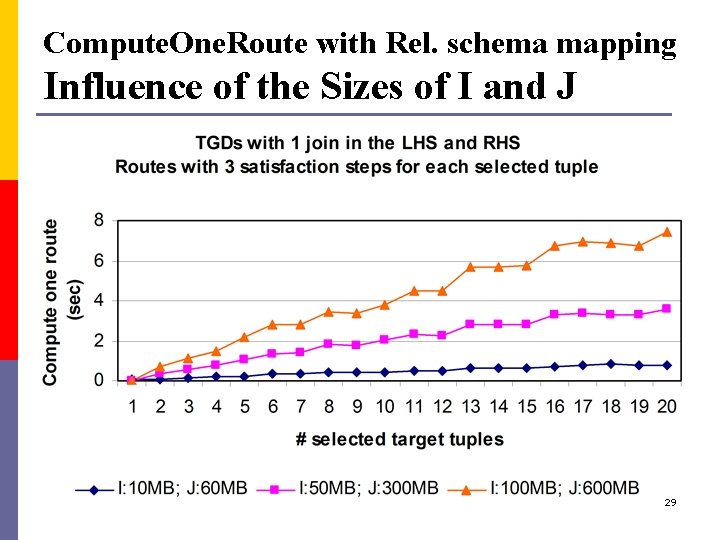
Compute. One. Route with Rel. schema mapping Influence of the Sizes of I and J 29

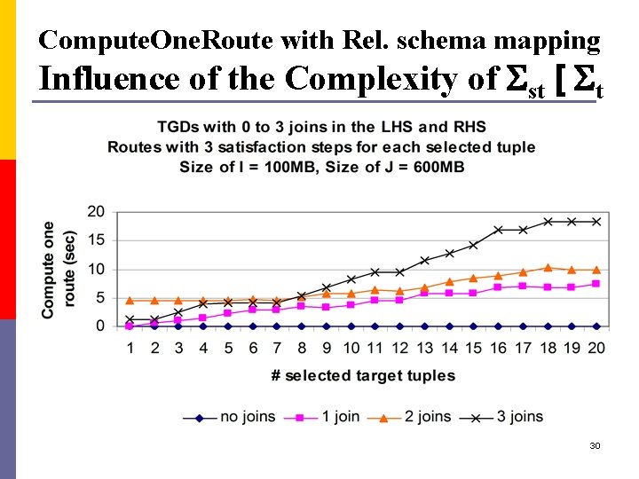
Compute. One. Route with Rel. schema mapping Influence of the Complexity of st [ t 30

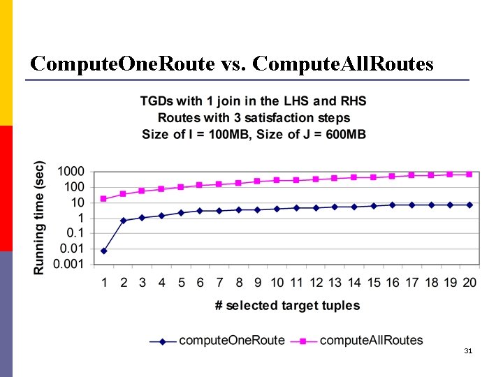
Compute. One. Route vs. Compute. All. Routes 31

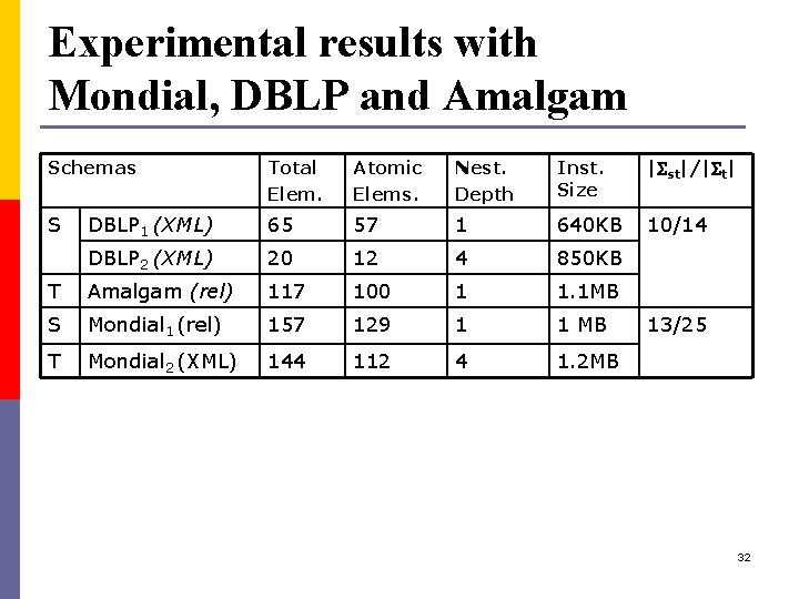
Experimental results with Mondial, DBLP and Amalgam Schemas Total Elem. Atomic Elems. Nest. Depth Inst. Size | st|/| t| S DBLP 1 (XML) 65 57 1 640 KB 10/14 DBLP 2 (XML) 20 12 4 850 KB T Amalgam (rel) 117 100 1 1. 1 MB S Mondial 1 (rel) 157 129 1 1 MB T Mondial 2 (XML) 144 112 4 1. 2 MB 13/25 32

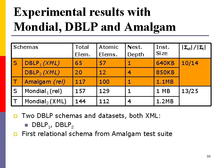
Experimental results with Mondial, DBLP and Amalgam Schemas Total Elem. Atomic Elems. Nest. Depth Inst. Size | st|/| t| S DBLP 1 (XML) 65 57 1 640 KB 10/14 DBLP 2 (XML) 20 12 4 850 KB T Amalgam (rel) 117 100 1 1. 1 MB S Mondial 1 (rel) 157 129 1 1 MB T Mondial 2 (XML) 144 112 4 1. 2 MB p p 13/25 Two DBLP schemas and datasets, both XML: n DBLP 1, DBLP 2 First relational schema from Amalgam test suite 33

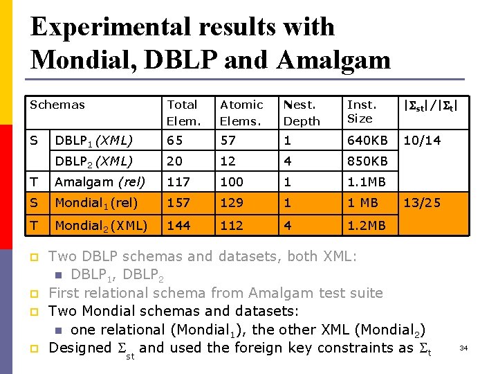
Experimental results with Mondial, DBLP and Amalgam Schemas Total Elem. Atomic Elems. Nest. Depth Inst. Size | st|/| t| S DBLP 1 (XML) 65 57 1 640 KB 10/14 DBLP 2 (XML) 20 12 4 850 KB T Amalgam (rel) 117 100 1 1. 1 MB S Mondial 1 (rel) 157 129 1 1 MB T Mondial 2 (XML) 144 112 4 1. 2 MB p p 13/25 Two DBLP schemas and datasets, both XML: n DBLP 1, DBLP 2 First relational schema from Amalgam test suite Two Mondial schemas and datasets: n one relational (Mondial 1), the other XML (Mondial 2) Designed st and used the foreign key constraints as t 34

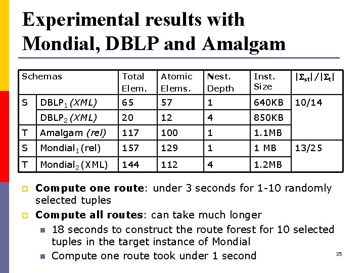
Experimental results with Mondial, DBLP and Amalgam Schemas Total Elem. Atomic Elems. Nest. Depth Inst. Size | st|/| t| S DBLP 1 (XML) 65 57 1 640 KB 10/14 DBLP 2 (XML) 20 12 4 850 KB T Amalgam (rel) 117 100 1 1. 1 MB S Mondial 1 (rel) 157 129 1 1 MB T Mondial 2 (XML) 144 112 4 1. 2 MB p p 13/25 Compute one route: under 3 seconds for 1 -10 randomly selected tuples Compute all routes: can take much longer n 18 seconds to construct the route forest for 10 selected tuples in the target instance of Mondial 35 n Compute one route took under 1 second

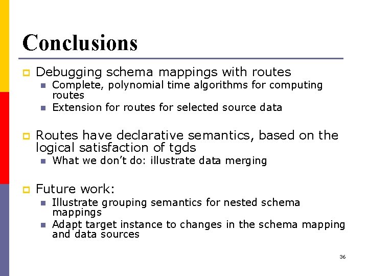
Conclusions p Debugging schema mappings with routes n n p Routes have declarative semantics, based on the logical satisfaction of tgds n p Complete, polynomial time algorithms for computing routes Extension for routes for selected source data What we don’t do: illustrate data merging Future work: n n Illustrate grouping semantics for nested schema mappings Adapt target instance to changes in the schema mapping and data sources 36

SPIDER: A Schema Mappings Debugger Demo group B Today 14: 00 -15: 30 Thursday 11: 00 -12: 30 p p Compute one/all routes Alternative routes Guided computation of routes Standard debugging features n n p Breakpoints “Watch” windows Schema-level routes 37

Thank you! 38

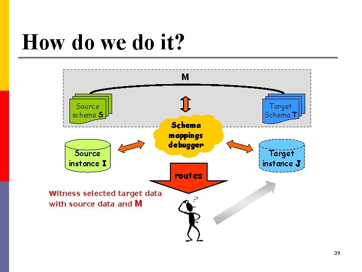
How do we do it? M Source schema S Source instance I Schema mappings debugger Target Schema T Target instance J routes Witness selected target data with source data and M 39

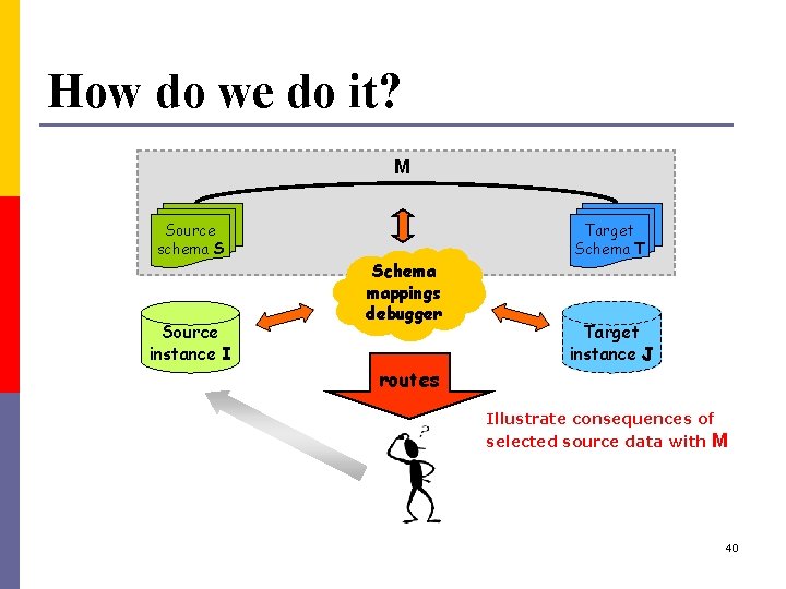
How do we do it? M Source schema S Source instance I Schema mappings debugger Target Schema T Target instance J routes Illustrate consequences of selected source data with M 40

Key Concept: ROUTES - describe the relationships between source and target data with the schema mapping M Source schema S Source instance I Schema mappings debugger Target Schema T Target instance J routes 41

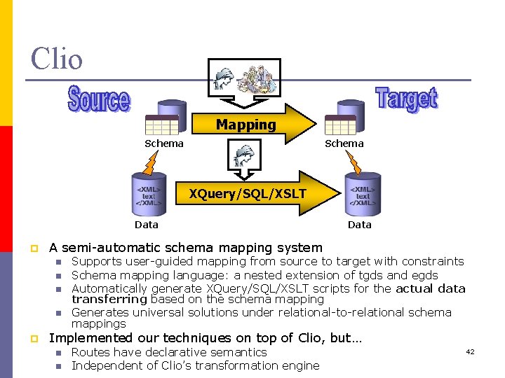
Clio Mapping Schema XQuery/SQL/XSLT Data p A semi-automatic schema mapping system n n p Data Supports user-guided mapping from source to target with constraints Schema mapping language: a nested extension of tgds and egds Automatically generate XQuery/SQL/XSLT scripts for the actual data transferring based on the schema mapping Generates universal solutions under relational-to-relational schema mappings Implemented our techniques on top of Clio, but… n n Routes have declarative semantics Independent of Clio’s transformation engine 42

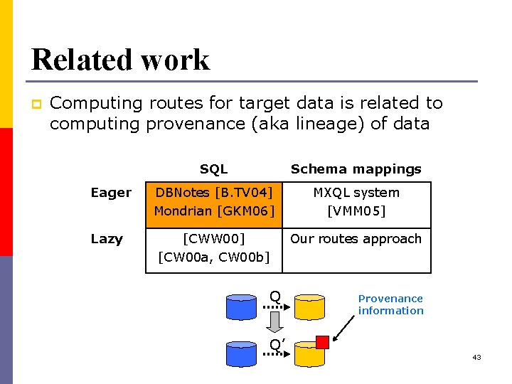
Related work p Computing routes for target data is related to computing provenance (aka lineage) of data Eager Lazy SQL Schema mappings DBNotes [B. TV 04] Mondrian [GKM 06] MXQL system [VMM 05] [CWW 00] [CW 00 a, CW 00 b] Our routes approach Q Q’ Provenance information 43

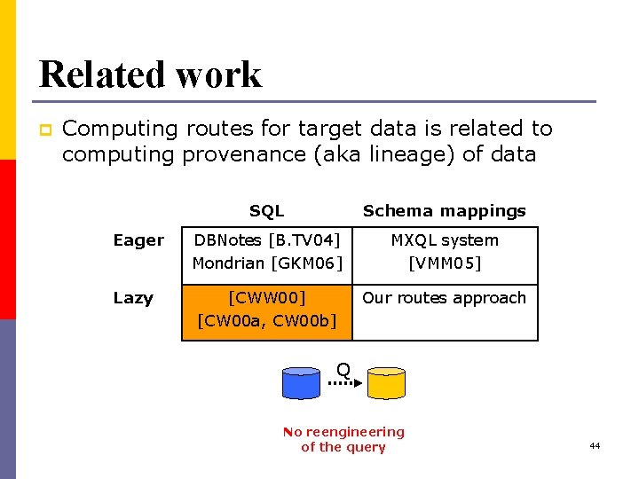
Related work p Computing routes for target data is related to computing provenance (aka lineage) of data Eager Lazy SQL Schema mappings DBNotes [B. TV 04] Mondrian [GKM 06] MXQL system [VMM 05] [CWW 00] [CW 00 a, CW 00 b] Our routes approach Q No reengineering of the query 44

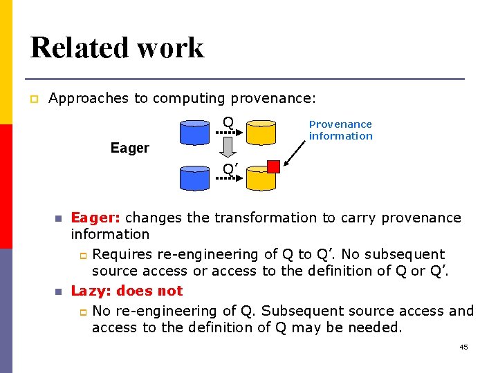
Related work p Approaches to computing provenance: Q Eager Provenance information Q’ n n Eager: changes the transformation to carry provenance information p Requires re-engineering of Q to Q’. No subsequent source access or access to the definition of Q or Q’. Lazy: does not p No re-engineering of Q. Subsequent source access and access to the definition of Q may be needed. 45

Related work p Computing routes for target data is related to computing provenance (aka lineage) of data Eager Lazy SQL Schema mappings DBNotes [BCTV 04] Mondrian [GKM 06] MXQL system [VMM 05] [CWW 00] [CW 00 a, CW 00 b] Our routes approach 46

Programming Languages vs. Schema Mappings p Debugging programming languages vs. debugging schema mappings n Procedural PL p We may have a specification (e. g. compute x 2 on input x) which completely determines the output § Well-defined notion of correct answer § The program is an implementation of the specification § If the correct answer is not obtained, there’s a bug – need to debug the implementation p However, the specification may also not be that concrete § E. g. , build a visual interface for … n Functional PL p p n Debugging is performed by analyzing a trace of the execution Declarative approach for debugging [Nilsson 94] Schema mapping IS the specification p p Infinite number of solutions consistent with the schema mapping Best we can do: look at the target instance – if something looks wrong (e. g. , the clients’ names are not copied to the target) go back to the schema mapping and try to refine it (or debug it) 47

Related Work: Computing Provenance of Data over SQL queries p Compute the provenance of relational data in a view in data warehouses [CWW 2000] n The provenance of a tuple t in a view is described as the tuples in the base tables that witness the existence of t Provenance answered using two reverse queries: R(a, b) : - R(a, b) Æ S(b, c) Æ a=1 Æ c=3 S(a, b) : - R(a, b) Æ S(b, c) Æ a=1 Æ c=3 T 1 3 View definition: T(a, c) : - R(a, b) Æ S(b, c) DB R SQL Schema mappings Eager DBNotes [BCTV 2004] [CTV 2005] MXQL system [VMM 2005] Lazy [CWW 2000] Our approach 48 S 1 2 2 3 4 5 6 7

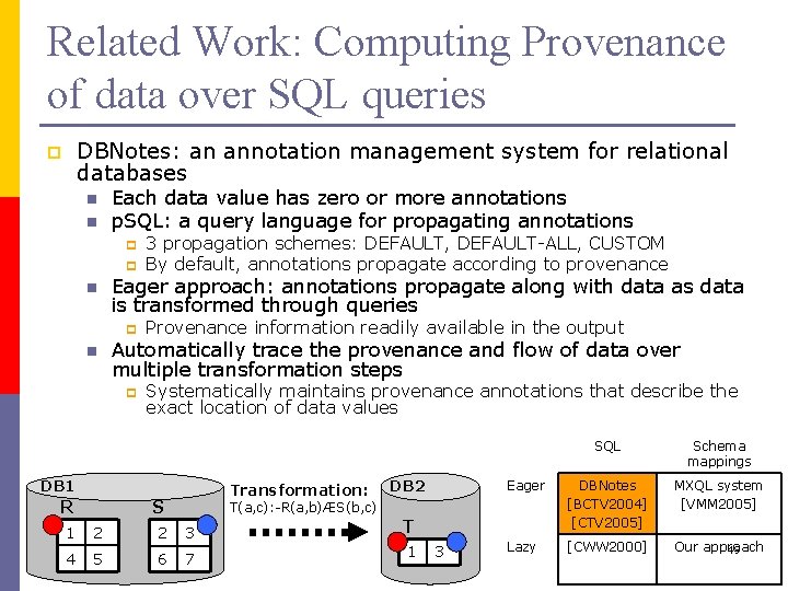
Related Work: Computing Provenance of data over SQL queries DBNotes: an annotation management system for relational databases p n n Each data value has zero or more annotations p. SQL: a query language for propagating annotations p p n Eager approach: annotations propagate along with data as data is transformed through queries p n 3 propagation schemes: DEFAULT, DEFAULT-ALL, CUSTOM By default, annotations propagate according to provenance Provenance information readily available in the output Automatically trace the provenance and flow of data over multiple transformation steps p Systematically maintains provenance annotations that describe the exact location of data values DB 1 R Transformation: S DB 2 SQL Schema mappings Eager DBNotes [BCTV 2004] [CTV 2005] MXQL system [VMM 2005] Lazy [CWW 2000] Our approach 49 T(a, c): -R(a, b)ÆS(b, c) 1 2 2 3 T 4 5 6 7 1 3

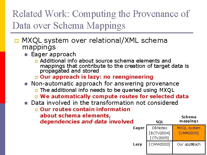
Related Work: Computing the Provenance of Data over Schema Mappings p MXQL system over relational/XML schema mappings n Eager approach p p n Non-automatic approach for answering provenance p p n Additional info about source schema elements and mappings that contribute to the creation of target data is propagated and stored Our approach is lazy: no reengineering The additional info needs to be queried using MXQL We automatically compute routes for selected data Data involved in the transformation not considered p Our routes contain information about schema elements, dependencies and data involved SQL Schema mappings Eager DBNotes [BCTV 2004] [CTV 2005] MXQL system [VMM 2005] Lazy [CWW 2000] 50 Our approach

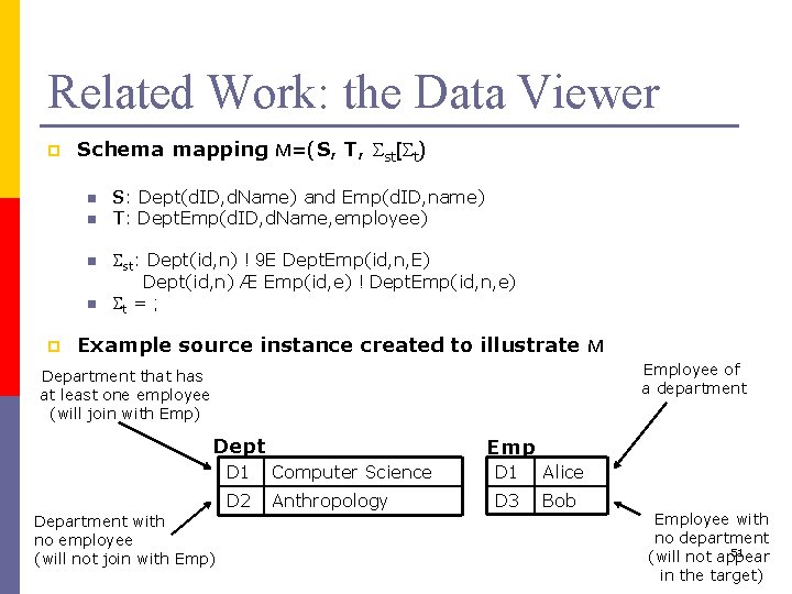
Related Work: the Data Viewer p Schema mapping M=(S, T, st[ t) n n p S: Dept(d. ID, d. Name) and Emp(d. ID, name) T: Dept. Emp(d. ID, d. Name, employee) st: Dept(id, n) ! 9 E Dept. Emp(id, n, E) Dept(id, n) Æ Emp(id, e) ! Dept. Emp(id, n, e) t = ; Example source instance created to illustrate M Employee of a department Department that has at least one employee (will join with Emp) Dept Department with no employee (will not join with Emp) Emp D 1 Computer Science D 1 Alice D 2 Anthropology D 3 Bob Employee with no department 51 (will not appear in the target)

Universal Solutions [FKMP 02] p Definition: Given two instances K 1 and K 2, a homomorphism h: K 1 → K 2 is a function h: Const[Var ! Const[Var such that: n n p Example: J 1={V(1, N 1), V(N 2, 2)}, J 2={V(1, 2)} n p p h(c) = c for all constants c For every fact R(a 1, …, an) 2 K 1, the fact R(h(a 1), …, h(an)) 2 K 2 h: J 1 ! J 2 is h={1 1, N 1 2, N 2 1, 2 2} Definition: Let M=(S, T, st[ t) be a schema mapping. If I is a source instance, then a universal solution for I is a solution J for I such that for every solution J’ for I, there exist a homomorphism h : J→J’ Example: st : R(x) ! 9 N V(x, N) U(x) ! 9 N V(N, x) n n n Source instance I={R(1), U(2)} J 2={V(1, 2)} is not a universal solution for I J 1={V(1, N 1), V(N 2, 2)} is a universal solution for I 52

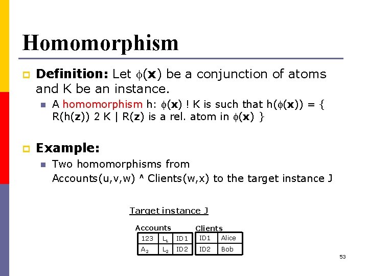
Homomorphism p Definition: Let (x) be a conjunction of atoms and K be an instance. n p A homomorphism h: (x) ! K is such that h( (x)) = { R(h(z)) 2 K | R(z) is a rel. atom in (x) } Example: n Two homomorphisms from Accounts(u, v, w) ^ Clients(w, x) to the target instance J Target instance J Accounts Clients 123 L 1 ID 1 Alice A 2 L 2 ID 2 Bob 53

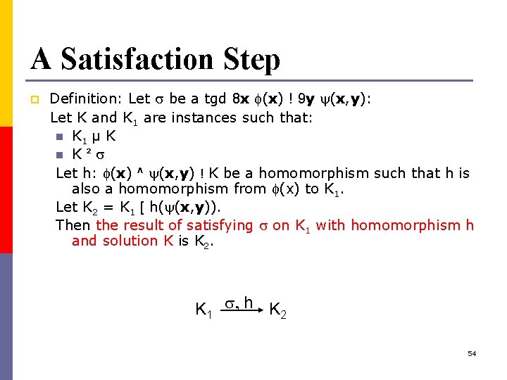
A Satisfaction Step p Definition: Let be a tgd 8 x (x) ! 9 y (x, y): Let K and K 1 are instances such that: n K 1 µ K n K ² Let h: (x) ^ (x, y) ! K be a homomorphism such that h is also a homomorphism from (x) to K 1. Let K 2 = K 1 [ h( (x, y)). Then the result of satisfying on K 1 with homomorphism h and solution K is K 2. K 1 , h K 2 54

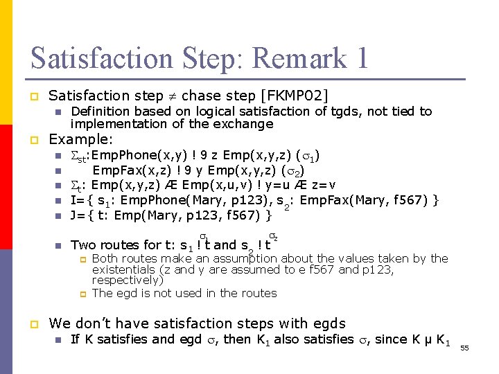
Satisfaction Step: Remark 1 p Satisfaction step chase step [FKMP 02] n p Definition based on logical satisfaction of tgds, not tied to implementation of the exchange Example: n n n st: Emp. Phone(x, y) ! 9 z Emp(x, y, z) ( 1) Emp. Fax(x, z) ! 9 y Emp(x, y, z) ( 2) t: Emp(x, y, z) Æ Emp(x, u, v) ! y=u Æ z=v I={ s 1: Emp. Phone(Mary, p 123), s 2: Emp. Fax(Mary, f 567) } J={ t: Emp(Mary, p 123, f 567) } 1 p p p 2 Two routes for t: s 1 ! t and s 2 ! t Both routes make an assumption about the values taken by the existentials (z and y are assumed to e f 567 and p 123, respectively) The egd is not used in the routes We don’t have satisfaction steps with egds n If K satisfies and egd , then K 1 also satisfies , since K µ K 1 55

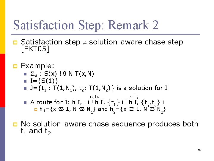
Satisfaction Step: Remark 2 p Satisfaction step solution-aware chase step [FKT 05] p Example: n n n st : S(x) ! 9 N T(x, N) I={S(1)} J={t 1: : T(1, N 1), t 2: T(1, N 2)} is a solution for I , h 1 n A route for J: h I, ; i ! h I, {t 1} i ! h I, {t 1, t 2} i p p , h 2 h 1={x 1, N N 1} and h 2={x 1, N N 2} No solution-aware chase sequence produces both t 1 and t 2 56

Computing all routes for target tuples p p The schema mapping M is fixed Input: n n n source instance I target instance J a set of target tuples Js µ J p Output: a route forest for Js that concisely represents all routes for Js p Algorithm idea: reverse chase n n n For each tuple R(a) in Js, consider every possible and h for witnessing R(a) Do the same for all target tuples encountered during the construction Do not consider the same tuple twice 57

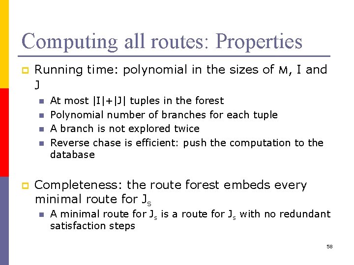
Computing all routes: Properties p Running time: polynomial in the sizes of M, I and J n n p At most |I|+|J| tuples in the forest Polynomial number of branches for each tuple A branch is not explored twice Reverse chase is efficient: push the computation to the database Completeness: the route forest embeds every minimal route for Js n A minimal route for Js is a route for Js with no redundant satisfaction steps 58

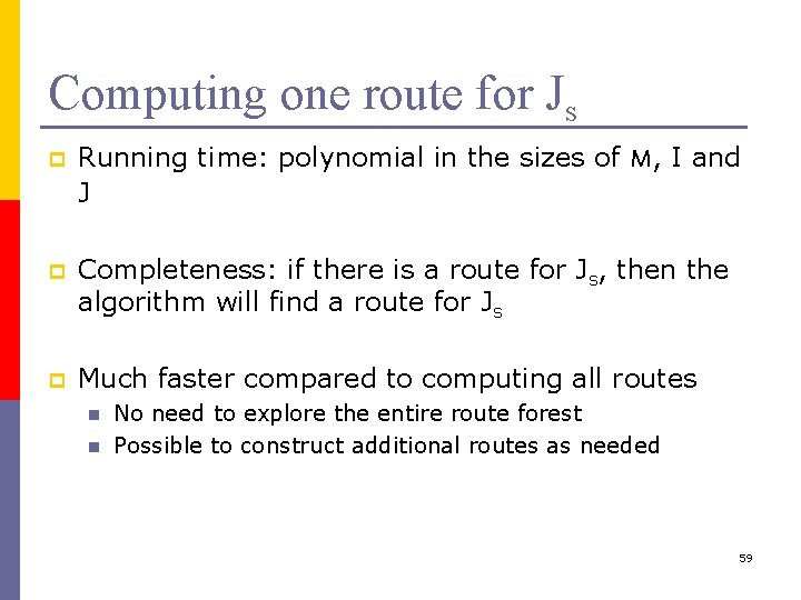
Computing one route for Js p Running time: polynomial in the sizes of M, I and J p Completeness: if there is a route for Js, then the algorithm will find a route for Js p Much faster compared to computing all routes n n No need to explore the entire route forest Possible to construct additional routes as needed 59

Some implementation details p Scalable approach: steps in routes are discovered by pushing computation to the database engine p Example: Source-to-target tgd: S(x, y) ! 9 U 9 V (T 1(x, U) ^ T 2(U, V, y)) n T 1(a, b) matched against RHS n LHS query: p S(a, y) is executed against the source instance using the db n RHS query: p T 1(a, b) ^ T 2(b, V, c) is executed against the target instance using the db n Each binding for y generates one RHS query n Design choice to decouple LHS and RHS queries p Extended for XML schema mappings 60

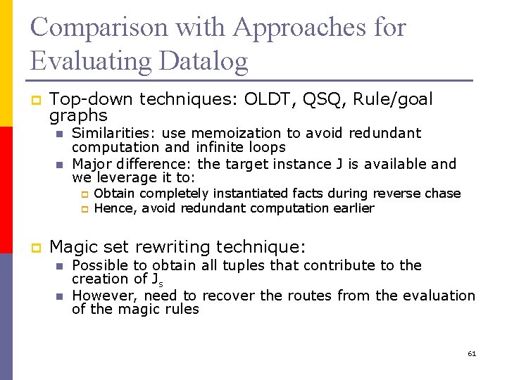
Comparison with Approaches for Evaluating Datalog p Top-down techniques: OLDT, QSQ, Rule/goal graphs n n Similarities: use memoization to avoid redundant computation and infinite loops Major difference: the target instance J is available and we leverage it to: p p p Obtain completely instantiated facts during reverse chase Hence, avoid redundant computation earlier Magic set rewriting technique: n n Possible to obtain all tuples that contribute to the creation of Js However, need to recover the routes from the evaluation of the magic rules 61

Top-down Example p n n p p 1: S 1(x, y) ! T 1(x, y) 2: S 2(x, y, u) ! T 2(x, y, u) t: n p T 3(1, 3) st: T 1(1, y) Æ T 2(y, 3, u) y 2 3: T 1(x, y) Æ T 2(y, z, u) ! T 3(x, z) I: S 1(1, 2) J: T 1(1, 2), T 3(1, 3) S 1(1, y) T 2(2, 3, u) y 2 S 2(2, 3, u) 62