Dealing with Uncertainty Navigation among Moving Obstacles A

Dealing with Uncertainty

Navigation among Moving Obstacles A robot with imperfect sensing must reach a goal location among moving obstacles (dynamic world) Goal 2

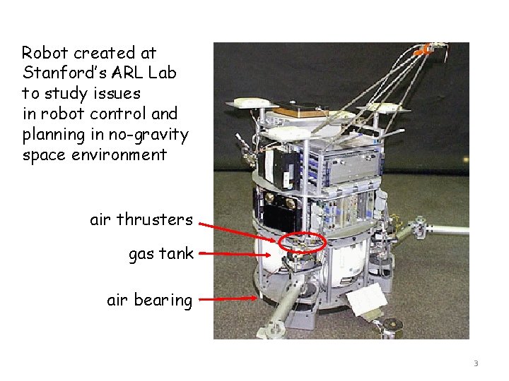
Robot created at Stanford’s ARL Lab to study issues in robot control and planning in no-gravity space environment air thrusters gas tank air bearing 3

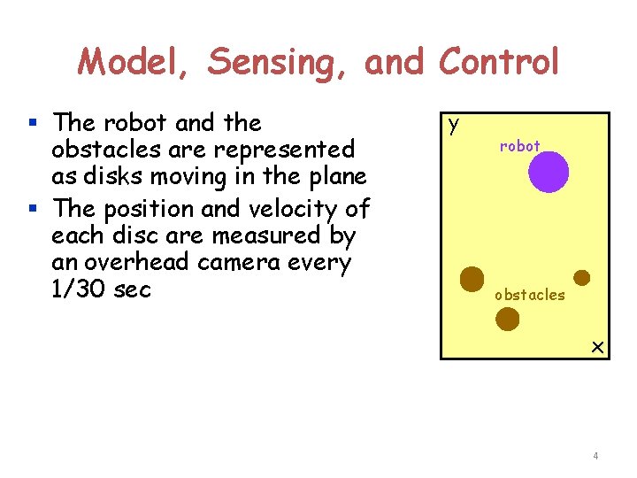
Model, Sensing, and Control § The robot and the obstacles are represented as disks moving in the plane § The position and velocity of each disc are measured by an overhead camera every 1/30 sec y robot obstacles x 4

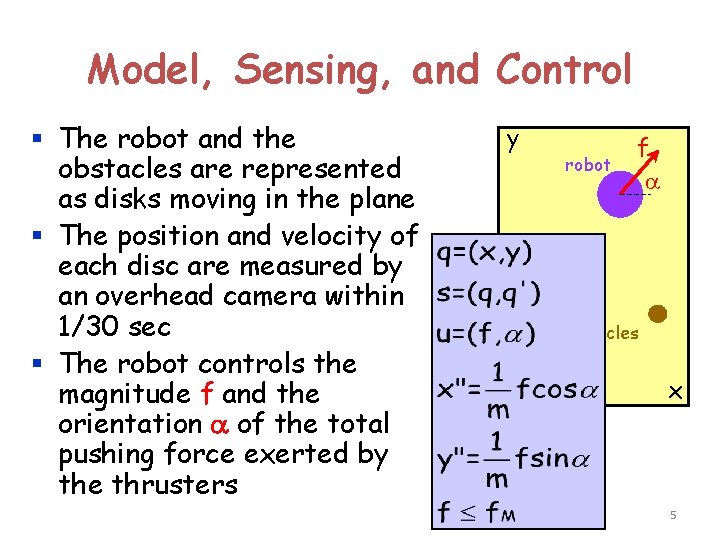
Model, Sensing, and Control § The robot and the obstacles are represented as disks moving in the plane § The position and velocity of each disc are measured by an overhead camera within 1/30 sec § The robot controls the magnitude f and the orientation a of the total pushing force exerted by the thrusters y robot f a obstacles x 5

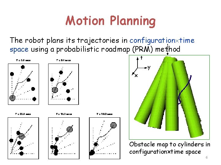
Motion Planning The robot plans its trajectories in configuration time space using a probabilistic roadmap (PRM) method t y x Obstacle map to cylinders in configuration time space 6

But executing this trajectory is likely to fail. . . 1) The measured velocities of the obstacles are inaccurate 2) Tiny particles of dust on the table affect trajectories and contribute further to deviation Obstacles are likely to deviate from their expected trajectories 3) Planning takes time, and during this time, obstacles keep moving The computed robot trajectory is not properly synchronized with those of the obstacles The robot may hit an obstacle before reaching its goal [Robot control is not perfect but “good” enough for the task] 7

But executing this trajectory is likely to fail. . . 1) The measured velocities of the obstacles are inaccurate 2) Tiny particles of dust on the table affect trajectories and contribute further to deviation Obstacles are likely to deviate from their expected trajectories 3) Planning takes time, and during this time, obstacles are moving The computed robot trajectory is not properly synchronized with those of the obstacles The robot may hit an obstacle before reaching its goal Planning must take both uncertainty in world [Robot control is not perfect but “good” enough for the task] state and time constraints into account 8

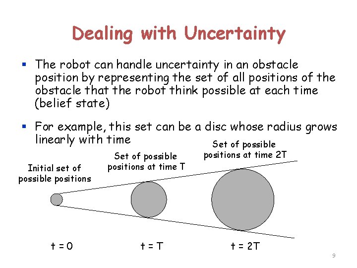
Dealing with Uncertainty § The robot can handle uncertainty in an obstacle position by representing the set of all positions of the obstacle that the robot think possible at each time (belief state) § For example, this set can be a disc whose radius grows linearly with time Set of possible Initial set of possible positions t=0 Set of possible positions at time T t=T positions at time 2 T t = 2 T 9

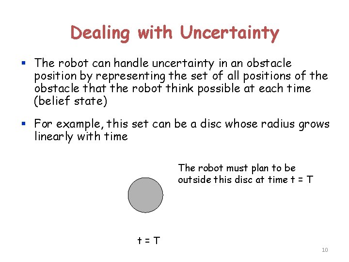
Dealing with Uncertainty § The robot can handle uncertainty in an obstacle position by representing the set of all positions of the obstacle that the robot think possible at each time (belief state) § For example, this set can be a disc whose radius grows linearly with time The robot must plan to be outside this disc at time t = T t=0 t=T t = 2 T 10

Dealing with Uncertainty § The robot can handle uncertainty in an obstacle position by representing the set of all positions of the obstacle that the robot think possible at each time (belief state) § For example, this set can be a disc whose radius grows linearly with time § The forbidden regions in configuration time space are cones, instead of cylinders § The trajectory planning method remains essentially unchanged 11

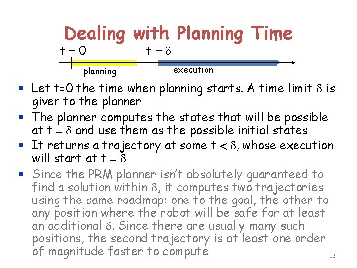
Dealing with Planning Time t=0 planning t=d execution § Let t=0 the time when planning starts. A time limit d is given to the planner § The planner computes the states that will be possible at t = d and use them as the possible initial states § It returns a trajectory at some t < d, whose execution will start at t = d § Since the PRM planner isn’t absolutely guaranteed to find a solution within d, it computes two trajectories using the same roadmap: one to the goal, the other to any position where the robot will be safe for at least an additional d. Since there are usually many such positions, the second trajectory is at least one order of magnitude faster to compute 12

Are we done? § Not quite ! § The uncertainty model may itself be incorrect, e. g. : • There may be more dust on the table than anticipated • Some obstacles have the ability to change trajectories § But if we are too careful, we will end up with forbidden regions so big that no solution trajectory will exist any more § So, it might be better to take some “risk” The robot must monitor the execution of the planned trajectory and be prepared to re-plan a new trajectory 13

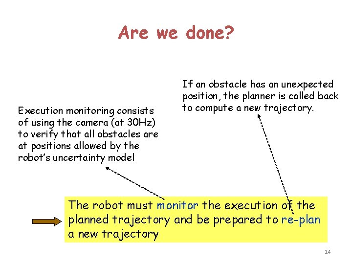
Are we done? Execution monitoring consists of using the camera (at 30 Hz) to verify that all obstacles are at positions allowed by the robot’s uncertainty model If an obstacle has an unexpected position, the planner is called back to compute a new trajectory. The robot must monitor the execution of the planned trajectory and be prepared to re-plan a new trajectory 14

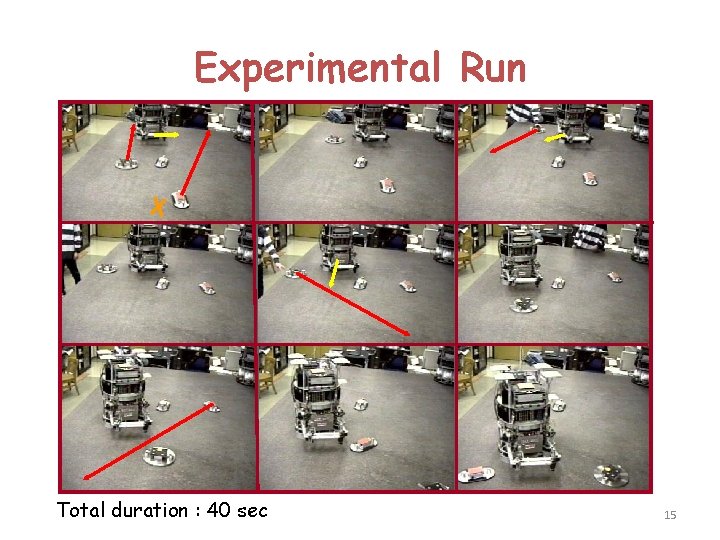
Experimental Run X Total duration : 40 sec 15

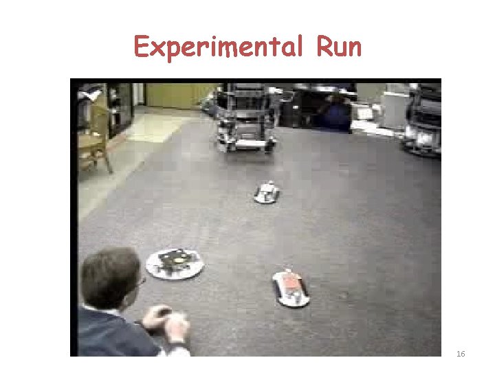
Experimental Run 16

Is this guaranteed to work? Of course not : § Thrusters might get clogged § The robot may run out of air or battery § The granite table may suddenly break into pieces § Etc. . . [Unbounded uncertainty] 17

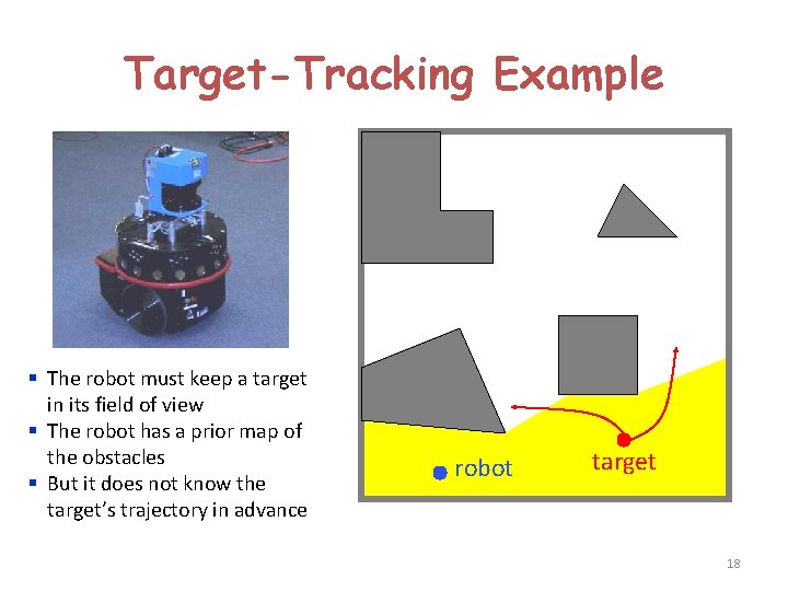
Target-Tracking Example § The robot must keep a target in its field of view § The robot has a prior map of the obstacles § But it does not know the target’s trajectory in advance robot target 18

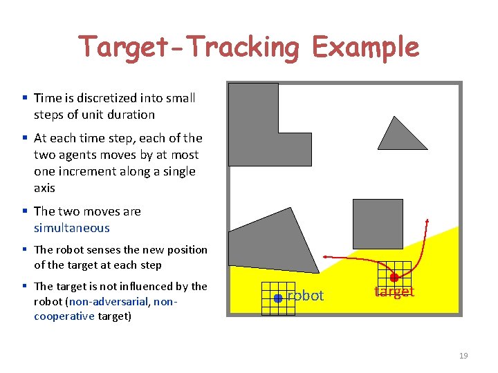
Target-Tracking Example § Time is discretized into small steps of unit duration § At each time step, each of the two agents moves by at most one increment along a single axis § The two moves are simultaneous § The robot senses the new position of the target at each step § The target is not influenced by the robot (non-adversarial, noncooperative target) robot target 19

Time-Stamped States (no cycles possible) ([i, j], [u, v], t) right • ([i+1, j], [u, v], t+1) • ([i+1, j], [u-1, v], t+1) • ([i+1, j], [u+1, v], t+1) • ([i+1, j], [u, v-1], t+1) • ([i+1, j], [u, v+1], t+1) § State = (robot-position, target-position, time) § In each state, the robot can execute 5 possible actions : {stop, up, down, right, left} § Each action has 5 possible outcomes (one for each possible action of the target), with some probability distribution [Potential collisions are ignored for simplifying the presentation] 20

Rewards and Costs The robot must keep seeing the target as long as possible § Each state where it does not see the target is terminal § The reward collected in every non-terminal state is 1; it is 0 in each terminal state [ The sum of the rewards collected in an execution run is exactly the amount of time the robot sees the target] § No cost for moving vs. not moving 21

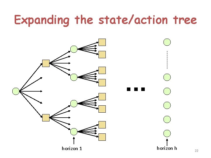
Expanding the state/action tree . . . horizon 1 horizon h 22

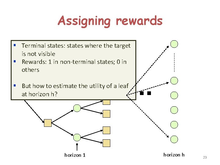
Assigning rewards § Terminal states: states where the target is not visible § Rewards: 1 in non-terminal states; 0 in others § But how to estimate the utility of a leaf at horizon h? horizon 1 . . . horizon h 23

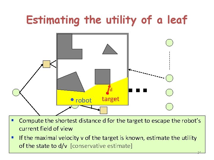
Estimating the utility of a leaf d robot target . . . § Compute the shortest distance d for the target to escape the robot’s current field of view § If the maximal velocity v of the target is known, estimate the utility of the state to d/v [conservative estimate] horizon 1 horizon h 24

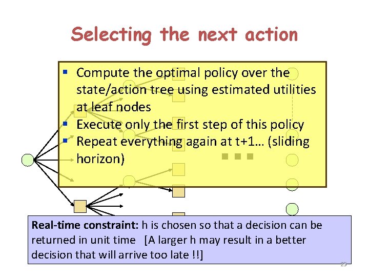
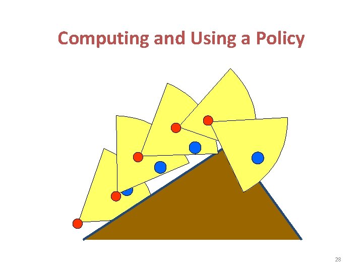
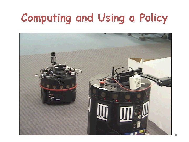
Selecting the next action § Compute the optimal policy over the state/action tree using estimated utilities at leaf nodes § Execute only the first step of this policy § Repeat everything again at t+1… (sliding horizon) . . . Real-time constraint: h is chosen so that a decision can be returned in unit time [A larger h may result in a better decision that will arrive too late !!] horizon h horizon 1 25

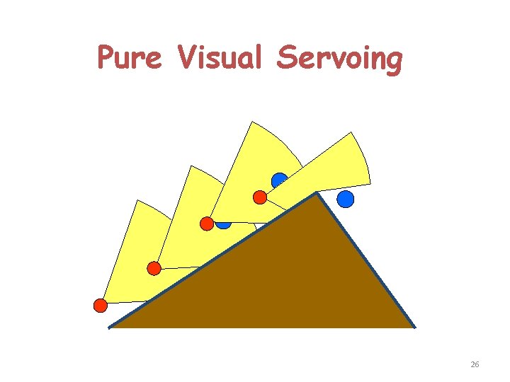
Pure Visual Servoing 26

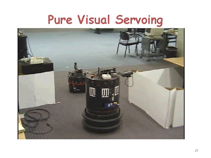
Pure Visual Servoing 27

Computing and Using a Policy 28

Computing and Using a Policy 29