Dealing with Exponential Problems Many important problems have

Dealing with Exponential Problems Many important problems have no polynomial solution but we still need to deal with them l The approach is to get "good" solutions in "efficient" time l Goodness and efficiency can be traded off to a certain degree l A number of powerful approaches l – Intelligent Search – Approximation Algorithms – Local Search – Stochastic Algorithms l The term "approximation algorithms" is often used for many of these approaches trying to approximate the optimal solution – Some intelligent search techniques will guarantee the optimal solution but the search is still exponential (as you would expect) CS 312 – Intelligent Search 1

Intelligent Search The full problem is made up of an exponential search space and thus exhaustive search is exponential l Informed (intelligent, "best-first") vs. uninformed search l Intelligent search seeks to reduce the number of states we actually search by one or both of the following: l – Pruning, as soon as possible, branches of the search tree which cannot lead to a solution – Trying first those branches which are most promising in hopes of finding a reasonable solution quickly, thus avoiding alternatives l Approaches – – Backtracking Branch and Bound Beam Search – Non optimal solution, but faster A* search CS 312 – Intelligent Search 2

Backtracking l Natural for decision search problems – Is there a solution or not l Example: SAT – Satisfiability – Does there exist a setting of Boolean variables which satisfies a particular CNF Boolean expression – – – – What is simple algorithm/complexity to solve it? NP-complete problem Verifiable in polynomial time – Easy to test What does full search tree look like? Backtracking allows us to prune branches Branch on arbitrary variable (e. g. w) Both leafs still possible, but when we branch on x, note that the leaf (w=0, x=1) is impossible so we can prune all subtrees of that node – can backtrack out of that dead-end (like pruning sub-tree below) CS 312 – Intelligent Search 3

Backtracking with SAT • Clauses in a node represent what still remains to be satisfied • Dropping a clause in a node means that the clause is satisfied • If we find any empty node (i. e. all clauses satisfied) then full expression is satisfiable • An empty clause signifies that the clause is not satisfiable and we can prune that path • If all leafs contain an empty clause then the expression is not satisfiable 4

Backtracking Algorithm l Backtracking is still exponential, but due to the pruning it is more practical in many cases – More room to increase the size of the problem before it becomes intractable CS 312 – Intelligent Search 5

Branch and Bound Similar to Backtracking but applied to optimization problems l Common and powerful technique for many tasks l For a minimization problem, we need an efficient/quick mechanism to generate an optimistic lowerbound(S) for a particular state S (or upperbound for maximization) l – From S we know that we could never get a better solution than lowerbound(S) – Note we want LB(S) as big as possible We keep track of the Best Solution So Far (BSSF) l If lowerbound(S) ≥ BSSF then we can prune S and not search anymore below it l The better (tighter) the bounding function the more we can prune the search l CS 312 – Intelligent Search 6

Bounding Function Example – 15 puzzle Want the least number of moves necessary to complete the puzzle l What does the search space look like? l What kind of bounding function could we use to help prune space? l – Must never over-estimate the actual optimum (is a lower-bound) – Can we do better? – The closer the bound can get to the actual optimum, the more we can prune – The bounding function should be relatively fast to compute – Would if bound estimate overestimated needed steps from the state? CS 312 – Intelligent Search 7

Branch and Bound Algorithm B&B returns the optimal solution Just like backtracking, B&B is still exponential, but often runs in relatively fast time due to pruning and depending on the quality of the bounding function l Before expanding a problem P S, make sure its' LB is still < BSSF, since BSSF may have been updated since P was put in the set S l Also, as a heuristic, could make S a priority queue with LB(P) as the key – always expand P with lowest LB as a heuristic l l – – To be optimal, all P with LB < BSSF must be expanded before we terminate In practice, we terminate sooner and return current non-optimal BSSF CS 312 – Intelligent Search 8

Beam Search A beam search is a semi-greedy state space search that only keeps a limited specified number (the beam width) of states in memory l When the state space exceeds the beam width, then all the states with the worst bound/heuristic value are dropped l Thus it is sub-optimal since the optimal solution may have been in one of the dropped states l More efficient in both time and space l – Memory is controlled explicitly by the beam width l Can make B&B a beam search by putting a max (beam width) on the number of states in S. Common approach. CS 312 – Intelligent Search 9

TSP B&B: Partial Path State Space n-1 branches from root, n-2 branches for each node at next level, etc. l The complete solutions are the (n-1)! leaves l – One for each possible path starting from node 1 l HUGE tree. We want an efficient bounding function for each state which could allow pruning to avoid searching all states – What is the loosest and what is the tightest bound? – What are some other bounds? CS 312 – Intelligent Search 10

TSP B&B: Partial Path State Space l Would like an efficient bounding function for each state which could allow pruning to avoid searching all states – Current partial distance + sum of the shortest edges leaving remaining nodes – Current partial distance + MST(remaining nodes) – etc. l Note that we also need a search space strategy that drills down to some final states so we can keep updating BSSF to allow better pruning CS 312 – Intelligent Search 11

TSP Project l l l As long as the bound is optimistic (≤ the optimal tour), branch and bound will return the optimal path for TSP if given sufficient time You will implement the following bounding approach for your project, together with an improved state space search We will not give you exact pseudo-code for this project, but will review approaches in the slides and make available some pertinent reading material n city problem – Directed graph version – can have asymmetric city distances A similar problem, Hamiltonian Cycle (also called a Rudrata Cycle), is also exponential – Does there exist a cycle which visits each node exactly once? CS 312 – Intelligent Search 12

Bound on TSP Tour 1 9 8 2 2 4 1 3 3 5 10 6 12 7 4 4 Hint: Every tour must leave every vertex and arrive at every vertex. Any proposals? 13

Bound on TSP Tour § Could use sum of smallest exiting edge from each vertex § or similarly, Could use sum of smallest entering edge into each vertex § Are these optimistic? § Could do even better if we can combine both § Sum them both? § Do one first, then sum in the residual of the other, given the first CS 312 – Intelligent Search 14

Bound on TSP Tour 1 9 8 2 2 4 1 3 3 5 10 6 12 7 4 4 What’s the cheapest way to leave each vertex? CS 312 – Intelligent Search 15

Bound on TSP Tour Initial rough bound = 8+2+3+6+1 = 20 1 9 8 2 2 4 1 3 3 5 6 10 12 7 4 4 Save the sum of those costs in the bound (as a first draft). CS 312 – Intelligent Search 16

Reduced Cost Matrix Rough draft bound = 20 1 9 -8=1 8 -8=0 2 2 4 1 3 3 5 10 6 12 7 4 4 For a given vertex, subtract the least departure edge cost from each edge leaving that vertex. This leaves the potential increased cost of taking a different edge in the reduced cost matrix. If we decide later to use edge (1, 2) instead of (1, 4), the cost would be only 1 more (9) than we already had (8). 17

Reduced Cost Matrix Rough draft bound = 20 0 1 1 0 2 2 0 0 3 5 9 0 6 1 1 4 Repeat for the other vertices. Now, let's find a tighter lower bound. Does the set of edges now having 0 residual cost (those making up our current bound) arrive at every vertex? – No. None into vertex 3 18

Bound on TSP Tour Rough draft bound = 20 0 1 1 0 2 2 0 0 3 5 9 0 6 1 1 4 We have to take an edge to vertex 3 from somewhere. Assume we take the cheapest currently available. 19

Bound on TSP Tour Bound = 21 1 1 0 0 2 1 0 0 3 5 9 0 6 0 1 4 Subtract this cheapest edge cost from all edges entering vertex 3 and add the cost to the bound. We do this for all vertices which did not have an inbound edge of 0 cost to complete our reduced cost matrix. 20 We have just tightened the bound.

The Bound § It will cost at least this much to visit all the vertices in the graph. § There is no cheaper way to get in and out of each vertex. § And, the edges in our reduced cost matrix are now labeled with the extra cost of choosing that edge in case we need to – will be helpful § Remember, the bound is not necessarily (and not usually) a solution, and for optimal minimization is always ≤ optimal solution CS 312 – Intelligent Search 21

Cost Matrix 1 9 2 2 4 6 7 3 3 1 8 5 10 4 4 12 ∞ 9 ∞ 8 ∞ ∞ ∞ 4 ∞ 2 ∞ 3 ∞ 4 ∞ ∞ 6 7 ∞ 12 1 ∞ ∞ 10 ∞ We can accomplish the steps of this approach using a cost matrix CS 312 – Intelligent Search 22

Reduced Cost Matrix 1 1 2 0 1 0 3 0 0 9 1 4 5 6 Reduce all rows (outgoing lengths) by subtracting the minimum path from the other path lengths. Sum the reduction amounts as we go to build the bound. ∞ 9 ∞ 8 ∞ ∞ ∞ 4 ∞ 2 ∞ 3 ∞ 4 ∞ ∞ 6 7 ∞ 12 1 ∞ ∞ 10 ∞ ∞ 1 ∞ 0 ∞ ∞ ∞ 2 ∞ 0 ∞ 1 ∞ ∞ 0 1 ∞ 6 0 ∞ ∞ 9 ∞ Initial rough bound = 8+2+3+6+1 = 20 23

Reduced Cost Matrix 1 1 2 0 1 0 3 0 0 9 1 4 5 6 Then reduce all columns (incoming lengths) by subtracting the minimum path lengths and adding them to the bound. Only column 3 reduces since it has no 0's. Now we have a tighter bound. Note that there is now at least one 0 in every row (out) and column (in). ∞ 1 ∞ 0 ∞ ∞ ∞ 2 ∞ 0 ∞ 1 ∞ ∞ 0 1 ∞ 6 0 ∞ ∞ 9 ∞ ∞ 1 ∞ 0 ∞ 0 ∞ 1 ∞ ∞ 0 0 ∞ 6 0 ∞ ∞ 9 ∞ final bound = 20 + 1 = 21 24

Reduced Cost Matrix Algorithm bound = 0 initially (or is the bound of the parent state) For each row in A Subtract the minimum cell value in the row from all cells in the row and add that value to the bound Then for each column in A Subtract the minimum cell value in the column from all cells in the column and add that value to the bound At that point every column and row will have at least one 0 entry and we will have the correct bound summed **Challenge** - Create the reduced cost matrix. What is the complexity? ∞ 8 12 4 What is the final lower Bound? 3 ∞ 7 1 2 6 ∞ 4 ∞ 3 5 ∞ A. B. C. D. E. bound = 0 13 10 9 12 None of the Above 25

Reduced Cost Matrix Algorithm bound = 0 initially (or is the bound of the parent state) For each row in A Subtract the minimum cell value in the row from all cells in the row and add that value to the bound Then for each column in A Subtract the minimum cell value in the column from all cells in the column and add that value to the bound At that point every column and row will have at least one 0 entry and we will have the correct bound summed **Challenge** - Create the reduced cost matrix. What is the complexity? – n 2 ∞ 8 12 4 ∞ 4 8 0 ∞ 4 6 0 3 ∞ 7 1 2 ∞ 6 0 2 ∞ 4 0 2 6 ∞ 4 0 4 ∞ 2 ∞ 3 5 ∞ ∞ 0 2 ∞ ∞ 0 0 ∞ bound = 0 bound = 4+1+2+3=10 bound = 10+2 = 12 26

Reduced Cost Matrix Algorithm § Could have done columns first and then rows § Which is better? § Still give a correct lower bound, though not necessarily the same reduced cost matrix and bound as the row first approach § Could try both, but then we have the trade-off of more time vs finding a better bound CS 312 – Intelligent Search 27

Initial BSSF Value: Infinite? A tighter value would lead to more initial pruning. Should be quick to calculate, but best if it is a reasonable value, since it may take a while before your first complete solutions finish and allow BSSF update and pruning 1 9 8 2 2 5 1 3 3 5 10 6 12 7 4 4 Don't use reduced matrix value because it will be lower than the optimal. BSSF is opposite of the bound in that it must be ≥ the optimal path (upper bound) - Want BSSF as small as possible, Optimal lies between lower bound and BSSF. Could simply try a few random legal paths and pick the best, or use greedy, etc. Be creative on this for your project. Can make a significant difference.

Random BSSF 1 9 5 1 8 2 2 3 3 Cost of random BSSF = 9+5+4+12+1 = 31 5 Want BSSF as low as possible and LB as high as possible 12 Optimal lies in between 10 6 7 4 4 CS 312 – Intelligent Search 29

State Space Search § The state space search approach defines the order in which children (or “successor”) states are expanded from a given state in the state space search (i. e. How we search through the tree). This is the search "frontier, " which in this case is stored in the priority queue. § We will introduce two approaches § The first assumes each state represents a partial path § § A link to a child state represents a path from the root city to the child We will arbitrarily make the first state represent city 1 § Children states in the search tree are generated by considering each path leaving the parent city in the TSP graph. We then calculate the reduced cost matrix for each child state and put child states whose bound is less than the BSSF on a priority queue where the bound is the PQ key § Do we need to use a priority queue? § Note that the initial reduced cost matrix is the same regardless of which node we start at CS 312 – Intelligent Search 30

Partial Path State Space CS 312 – Intelligent Search 31

State Space Search – Partial Path State 1 (21) 1 9 1 8 2 2 10 6 3 4 5 12 7 3 4 4 ∞ 1 ∞ 0 ∞ ∞ ∞ 1 ∞ 0 ∞ 1 ∞ ∞ 0 0 ∞ 6 0 ∞ ∞ 9 ∞ (1, 2) State 2 State 3 ∞ 1 ∞ 0 ∞ ∞ ∞ 1 ∞ 0 ∞ 1 ∞ ∞ 0 0 ∞ 6 0 ∞ ∞ 9 ∞ S 6 S 7 S 8 (1, 3) BSSF = 31 Don't confuse search state number with city number (1, 4) (1, 5) State 4 State 5 What changes? bound = 21 + ? S 9 S 10 S 11 S 12 S 13 S 14 S 15 S 16 S 17 32

State Space Search – Partial Path State 1 (21) 1 9 1 8 2 2 10 6 3 4 5 12 7 3 4 4 ∞ 1 ∞ 0 ∞ ∞ ∞ 1 ∞ 0 ∞ 1 ∞ ∞ 0 0 ∞ 6 0 ∞ ∞ 9 ∞ (1, 2) State 2 State 3 ∞ ∞ ∞ ∞ 1 ∞ 0 ∞ ∞ ∞ 1 ∞ ∞ ∞ 0 ∞ 6 0 ∞ ∞ 9 ∞ S 6 S 7 S 8 (1, 3) BSSF = 31 Don't confuse search state number with city number (1, 4) (1, 5) State 4 State 5 What changes? (row: from column: to) bound = 21 + 1 (cost of edge) + ? First set "from row" and "to column" = ∞ also for selected edge (i, j), set (j, i) = ∞ S 9 S 10 S 11 S 12 S 13 S 14 S 15 S 16 S 17 33

State Space Search – Partial Path State 1 (21) 1 9 1 8 2 2 10 6 3 4 5 12 7 3 4 4 ∞ 1 ∞ 0 ∞ ∞ ∞ 1 ∞ 0 ∞ 1 ∞ ∞ 0 0 ∞ 6 0 ∞ ∞ 9 ∞ (1, 2) State 2 State 3 ∞ ∞ ∞ ∞ 1 ∞ 0 ∞ ∞ ∞ 0 ∞ 6 0 ∞ ∞ 9 ∞ S 6 S 7 S 8 (1, 3) BSSF = 31 Don't confuse search state number with city number (1, 4) (1, 5) State 4 State 5 What changes? (row: from column: to) bound = 21 + 1 = 23 = prev bound + remaining_path_cost(1, 2) + cost of reducing the updated cost matrix S 9 S 10 S 11 S 12 S 13 S 14 S 15 S 16 S 17 34

State Space Search – Partial Path State 1 (21) 1 9 8 2 2 4 1 5 10 6 3 12 7 3 4 4 ∞ 1 ∞ 0 ∞ ∞ ∞ 1 ∞ 0 ∞ 1 ∞ ∞ 0 0 ∞ 6 0 ∞ ∞ 9 ∞ (1, 3) (1, 2) State 2 (21+1+1=23) State 3 (21+∞+1=∞) BSSF = 31 Don't confuse search state number with city number (1, 4) (1, 5) State 4 (21+0+0=21) State 5 (21+∞+∞=∞) ∞ ∞ ∞ ∞ ∞ ∞ 1 ∞ 0 ∞ ∞ 1 ∞ 0 ∞ ∞ 0 ∞ ∞ ∞ ∞ 0 ∞ 6 ∞ 0 ∞ ∞ 6 ∞ 0 0 ∞ ∞ 9 ∞ 0 ∞ ∞ ∞ ∞ 9 ∞ S 6 S 7 S 8 S 9 S 10 S 11 S 12 S 13 S 14 S 15 S 16 S 17 35

State Space Search § To create each new state, start with the bound for the parent state and § Add the residual cost of the new path § Set to infinity paths which can no longer be used (row of from-state, column of to-state, and tofrom state) § Reduce the new matrix and add the cost of reduction § States 3 and 5 will be pruned § States 2 and 4 will be enqueued and state 4 (with the lowest bound 21) will be the first on the queue and the next state expanded if using a priority queue § Adjust BSSF? - Not until we have a complete solution which is better § Number of remaining edges in the graph decrease at each level of the tree 36

State Space Search State 4 (21) 1 9 8 2 2 4 1 3 5 10 6 12 7 3 4 4 ∞ ∞ ∞ ∞ 1 ∞ 0 ∞ ∞ 0 0 ∞ 6 0 ∞ ∞ BSSF = 31 Went from city 1 to 4 37

**Challenge Question** State 4 (21) 1 9 8 2 2 4 1 5 10 6 3 12 7 3 4 4 (4, 2) ∞ ∞ ∞ ∞ 1 ∞ 0 ∞ ∞ 0 0 ∞ 6 0 ∞ ∞ (4, 3) State 12 (21+0+∞=∞) State 13 (21+…) ∞ ∞ ∞ ∞ 0 ∞ ∞ • • • BSSF = 31 (4, 5) State 14 (21+… Show the updated matrices for states 13 and 14 What are their lower bounds? Which ones go on the queue and which state will be expanded next? 38

State Space Search State 4 (21) 1 9 8 2 2 4 1 5 10 6 3 12 7 3 4 4 ∞ ∞ ∞ ∞ 1 ∞ 0 ∞ ∞ 0 0 ∞ 6 0 ∞ ∞ (4, 3) (4, 2) State 12 (21+0+∞=∞) State 13 (21+0+0=21) BSSF = 31 (4, 5) State 14 (21+6+1)=28 ∞ ∞ ∞ ∞ ∞ 0 ∞ ∞ ∞ ∞ ∞ 0 ∞ ∞ ∞ ∞ ∞ ∞ 0 ∞ ∞ ∞ ∞ 0 ∞ ∞ 13 and 14 will be put on the queue with State 13 the lowest 39

State Space Search State 13 (21) Path so far 1, 4, 3 1 9 8 2 2 4 1 3 5 10 6 12 7 3 4 4 ∞ ∞ ∞ ∞ ∞ 0 ∞ ∞ (3, 2) BSSF = 31 (3, 5) (21+∞+∞)=∞ (21+0+0=21) ∞ ∞ ∞ ∞ 0 ∞ ∞ ∞ ∞ ∞ ∞ ∞ 0 ∞ ∞ ∞ ∞ Just the first state is put in the queue and it will then select path 2 -5 with no new added cost. The last step will be the path 5 -1 which also has no added cost 40

Search Tree for Partial Path Search Complete path at bottom state is 1 – 4 – 3 – 2 – 5 – 1 Total Distance = 21 b=21 1 -to-2 b=23 1 -to-4 b=21 4 -to-2 b=∞ 4 -to-3 b=21 4 -to-5 b=28 3 -to-2 b=21 2 -to-5 5 -to-1 Once we hit the first complete solution, BSSF is updated to 21. In this case the two states on the queue (23, 28) will be pruned as soon as they are dequeued, leaving the queue empty and the algorithm will stop and return 21 If there had been states on the queue with a bound lower than the updated BSSF, then processing would have continued Note perfect efficiency! We never expanded a node that was not on the optimal path CS 312 – Intelligent Search 41

B&B Complexity l l B&B is notoriously hard for finding exact complexity Worst case complexity is easy by assuming we explore most nodes in the search tree which is in general O(bound(n) * bn), where b is the average branching factor, n is the depth of the tree, and bound(n) is the complexity of finding the bound at each node – Our partial path TSP B&B worst case time and space complexity is an impressive O(n 2(n+1)!) l However, we expect the pruning in B&B to keep the average branching factor and average depth much smaller, thus exploring a small subset of the search tree – Our partial path does require full depth n for each solution reached B&B is still exponential in n and how much smaller than worse case depends on the problem and the quality and efficiency of the bounding function and search space strategy. Real gain is how small a percentage of full tree did you need to explore. l Empirically, B&B can do quite well l – Often combine with beam search to limit the complexity CS 312 – Intelligent Search 42

Improved State Space Search l We used a priority queue so that the state with the best (lowest) bound can be chosen when it is time to expand a new state – For the partial path state space search this can lead to a fairly broad (breadth-first) search frontier as shallower nodes tend to have lower bounds since bounds increase monotonically with depth – All O(n) child states are calculated (and many put in the queue) each time a state is expanded – Leads to a large number of states in the priority queue – Also, BSSF is not updated until a completed path node (leaf) is reached which could be a while for large n l We prefer a state space search that "drills deeper" leading to finding complete paths which will update the BSSF sooner and lead to earlier pruning CS 312 – Intelligent Search 43

Digging Deeper In your project, you will note that as the number of cities grow and you hit your time limit, your B&B will almost always return your initial BSSF path l This is because you are always expanding the node with the lowest score and thus the first actual solution you find, will often be the optimal solution (more of a breadth first search) l However for large n it will take a long time to get the first solution as you continually expand nodes higher in the tree l For your project you will try some approaches to encourage "drilling down" in order to get earlier improved BSSF values l – Finding a balance, round-robin, adjust after initial drilling? , etc. l Note that this should not sacrifice optimality within the time limit, but when the time limit is exceeded (non-optimal result), you could get a better result than the initial BSSF path – You can also gain advantages from early pruning due to tighter BSSFs CS 312 – Intelligent Search 44

Branch and Bound Project l Implement a time bound – One advantage of Branch and Bound is you can always just return the BSSF if time runs out – Hopefully its not the initial one Use slide example for debugging if you want l Different City distributions l – Easy: symmetric city distances – Normal: non-symmetric city distances – Hard: non-symmetric city distances and some infinite distances l Use will use the hard setting for all of your reporting You will report total numbers of states created, max stored, and states pruned (not substates below which is real gain) l Start early! – This program entails somewhat more than previous ones l CS 312 – Intelligent Search 45

Include/Exclude State Space Search Include/Exclude approach can improve TSP performance compared to the partial path approach and we used to use it for your project as it digs deeper more naturally - Homework l We'll use the same reduced cost matrix bounding function, though any bounding function could be used l We do not choose an initial city to start at; we just have the initial reduced cost matrix tied to the initial search state l The search tree will be a binary tree with the decision based on whether a particular edge is in the final solution or out of it l Include edge (i, j) Exclude edge (i, j) Note that the left (include) child reduces our subsequent options to paths of length n-1 while the right (exclude) child still requires us to find a path of length n, which cannot include edge (i, j) l Which edge would you choose? l CS 312 – Intelligent Search 46

Include/Exclude State Space Search Include edge (i, j) Exclude edge (i, j) We want to include the best edges (usually very short edges between cities). Solutions including the good edges usually are better and have lower bounds. Solutions which exclude good edges are usually worse and have higher lower bounds and will be pruned. l Thus, rather than just shortest edges, we want edges which lead to lower bounds on the include side and high lower bounds on the exclude side l Choose the edge that maximizes the difference: b(exclude) - b(include), where b(s) is the lower bound function for the state l We hope this leads to "digging deep" down the include side to get new BSSFs, while leading to quick pruning down the exclude side l CS 312 – Intelligent Search 47

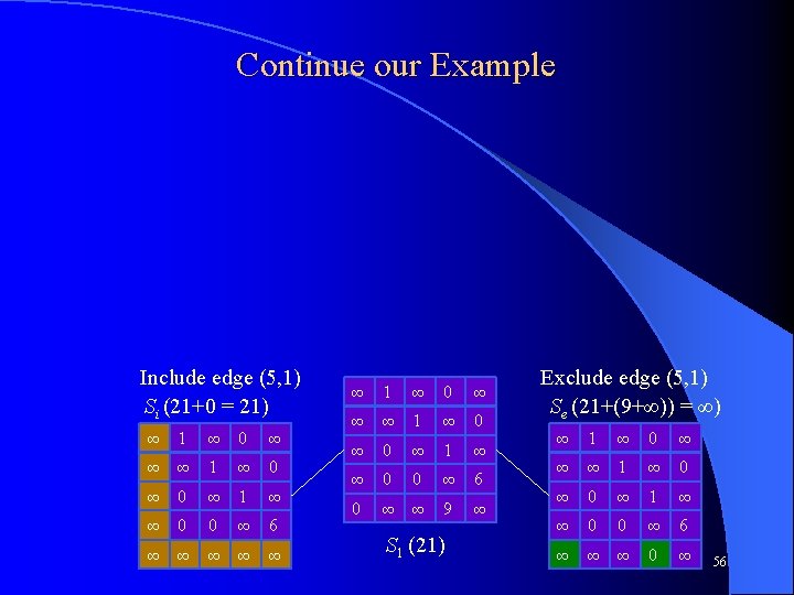
Include/Exclude State Space Search Include edge (i, j) Exclude edge (i, j) Si l l l Se How do we select the best of the up to n 2 edges in our graph? Select from those in our current reduced cost matrix – still n 2 Including 0 -cost paths tends to keep include bounds low, while excluding 0 cost paths tends to increase exclude bounds, (and always at least one 0 cost path available in every row not yet travelled from), thus we will only consider 0 -cost paths – Just O(n) edges to consider Select the 0 -cost edge which maximizes b(Se) – b(Si) Let's consider one of our 0 -cost edges: (5, 1) – brown fill represents included path, green represents updates Si (21+? ) ∞ 1 ∞ 0 ∞ ∞ ∞ 1 ∞ 0 ∞ 1 ∞ ∞ 0 0 ∞ 6 ∞ ∞ ∞ 1 ∞ 0 ∞ 1 ∞ ∞ 0 0 ∞ 6 0 ∞ ∞ 9 ∞ S 1 (21) Se (21+? ) ∞ 1 ∞ 0 ∞ ∞ ∞ 1 ∞ 0 ∞ 1 ∞ ∞ 0 0 ∞ 6 ∞ ∞ ∞ 0 ∞ 48

Which Edge is Best? How do we find the best edge to chose? l The candidate (0 -cost) edges are (1, 4), (2, 5), (3, 2), (4, 3), (5, 1) l We just try them all (O(n)) to see which maximizes b(Se) – b(Si) l Note that after setting Se(i, j) = ∞ that l b(Se) = b(Sparent) + min(rowi) + min(columnj) We reduce both states Se and Si and put them in the priority queue (as long as their bound < BSSF) and then take next lowest state off the queue Si and children of Si must keep track that (5, 1) is part of its final path Note that we could free or reuse memory for S 1 at this point Include edge (5, 1) Si (21+0 = 21) ∞ 1 ∞ 0 ∞ ∞ ∞ 1 ∞ 0 ∞ 1 ∞ ∞ 0 0 ∞ 6 ∞ ∞ ∞ 1 ∞ 0 ∞ 1 ∞ ∞ 0 0 ∞ 6 0 ∞ ∞ 9 ∞ S 1 (21) Exclude edge (5, 1) Se (21+(9+∞)) = ∞) ∞ 1 ∞ 0 ∞ ∞ ∞ 1 ∞ 0 ∞ 1 ∞ ∞ 0 0 ∞ 6 ∞ ∞ ∞ 0 ∞ 49

Premature Cycles An issue which must be dealt with: Premature cycles l If edge (i, j) is included, then edge (j, i) can not be used and must be marked as infinite in Si l l In the case below (5, 1), (1, 5) already happened to be infinite, but normally may not be Include edge (5, 1) Si (21) ∞ 1 ∞ 0 ∞ ∞ ∞ 1 ∞ 0 ∞ 1 ∞ ∞ 0 0 ∞ 6 ∞ ∞ ∞ 1 ∞ 0 ∞ 1 ∞ ∞ 0 0 ∞ 6 0 ∞ ∞ 9 ∞ S 1 (21) Exclude edge (5, 1) Se (∞) ∞ 1 ∞ 0 ∞ ∞ ∞ 1 ∞ 0 ∞ 1 ∞ ∞ 0 0 ∞ 6 ∞ ∞ ∞ 0 ∞ 50

Premature Cycles In fact, we must set to infinity all edges (k, m) which would complete a consecutive partial solution (of length < n) starting from j and ending at i. In the picture below assume n > 5 and that each white arrow is an included edge along an include state-space path and we then add the edge i to j. We must set to infinity the cells in the reduced cost matrix corresponding to all the red edges shown. l These exclusions may cause further reduction of Si which must be considered when calculating the reduced cost matrix for Si. This is good as it is more likely to tighten bounds and prune states! l a b i j z 51

Premature Cycles In fact, we must set to infinity all edges (k, m) which would complete a consecutive partial solution (of length < n) starting from j and ending at i. In the picture below assume n > 5 and that each white arrow is an included edge along an include state-space path and we then add the edge i to j. We must set to infinity the cells in the reduced cost matrix corresponding to all the red edges shown. l These exclusions may cause further reduction of Si which must be considered when calculating the reduced cost matrix for Si. This is good as it is more likely to tighten bounds and prune states! l a b i j z 52

Premature Cycles In fact, we must set to infinity all edges (k, m) which would complete a consecutive partial solution (of length < n) starting from j and ending at i. In the picture below assume n > 5 and that each white arrow is an included edge along an include state-space path and we then add the edge i to j. We must set to infinity the cells in the reduced cost matrix corresponding to all the red edges shown. l These exclusions may cause further reduction of Si which must be considered when calculating the reduced cost matrix for Si. This is good as it is more likely to tighten bounds and prune states! l a b i j z 53

Avoiding Premature Cycles If you add edge (i, j) then you need to set to infinity (delete) some edges that are subsequently impossible and might lead to a premature cycle. The vectors Entered and Exited are initialized to -1 before processing is started and updated as processing continues. This should do the job, since other premature cycles are prevented by our matrix updates, but you may do it however you want. function delete. Edges (M: matrix, i, j: int): matrix Entered[j] = i Exited[i] = j start = i end = j // The new edge may be part of a partial solution. Go to the end of that solution. while (Exited[end] != -1) do end = exited[end] // Similarly, go to the start of the new partial solution. while (entered[start] != -1) do start = entered[start] // Delete the edges that would make partial cycles, unless we’re ready to finish the tour if (partial_path_length < n-1) then Repeat Until (start = j) M[end, start] = infinity M[j, start] = infinity start = exited[start] return M CS 312 – Intelligent Search 54

Premature Cycles in Partial Path For the Partial Path State Space Search you do not need to worry about premature cycles l The search space does not allow it as each path down the tree has no cycles l When your path hits depth n, the only path remaining will be an edge from the leaf node back to city 1 to complete the cycle l CS 312 – Intelligent Search 55

One More Iteration l Possible 0 -cost edges are? S 2 (21) ∞ 1 ∞ 0 ∞ ∞ ∞ 1 ∞ 0 ∞ 1 ∞ ∞ 0 0 ∞ 6 ∞ ∞ ∞ includes edge (5, 1) 57

One More Iteration l Possible 0 -cost edges are (1, 4), (2, 5), (3, 2), (4, 3) S 2 (21) ∞ 1 ∞ 0 ∞ ∞ ∞ 1 ∞ 0 ∞ 1 ∞ ∞ 0 0 ∞ 6 ∞ ∞ ∞ includes edge (5, 1) 58

One More Iteration Possible 0 -cost edges are (1, 4), (2, 5), (3, 2), (4, 3) l Edge (2, 5) maximizes b(Se) – b(Si) l To avoid premature cycles in Si we set which cells to ∞? Note (1, 5) was set to ∞ in the previous iteration l S 2 (21) ∞ 1 ∞ 0 ∞ ∞ ∞ 1 ∞ 0 ∞ 1 ∞ ∞ 0 0 ∞ 6 ∞ ∞ ∞ includes edge (5, 1) 59

One More Iteration Possible 0 -cost edges are (1, 4), (2, 5), (3, 2), (4, 3) l Choosing (2, 5) maximizes b(Se) – b(Si) l To avoid premature cycles in Si we set (5, 2) (no change in this case) and (1, 2) to ∞ - Why? note (1, 5) was set to ∞ in the previous iteration l Both states are added to the queue assuming BSSF is 31 as before l Include edge (2, 5) Si (21+0=21) Now includes edges (5, 1) and (2, 5) ∞ ∞ ∞ 0 ∞ 1 ∞ ∞ 0 0 ∞ ∞ ∞ ∞ S 2 (21) ∞ 1 ∞ 0 ∞ ∞ ∞ 1 ∞ 0 ∞ 1 ∞ ∞ 0 0 ∞ 6 ∞ ∞ ∞ CS 312 – Intelligent Search Exclude edge (2, 5) Se (21+(6+1)=28) ∞ 1 ∞ 0 ∞ ∞ ∞ 0 ∞ 1 ∞ ∞ 0 0 ∞ ∞ ∞ includes edge (5, 1) 60

Include/Exclude Search Different initial search tree than partial path, but still factorial number of all possible solutions at leaves l Could use the same high level state space search as Partial Path (favor nodes with low bounds and still do some digging deep) l – – – Both typically use priority queue But they employ different expansion routines Rather than expand each possible next city path (partial path), expand into two new children Pi by including/excluding the edge which maximizes b(Se) – b(Si) CS 312 – Intelligent Search 61

Search Space for Include/Exclude BSSF = 31 initially 21 include (5, 1) exclude (5, 1) ∞ - not added to queue 21 include (2, 5) 21 include (1, 4) exclude (2, 5) 28 exclude (1, 4) 21 include (3, 2) 21 include (4, 3) 21 ∞ - not added Note that no particular node was constrained to be the beginning node of a path After updating BSSF to 21 all remaining states in priority queue will be pruned 62

Include Exclude B&B Complexity Same basic exponential complexity issues and values as partial path l Finding the bound is O(n 3) rather than O(n 2) since each node expansion tests n possible edges and for each alternative does a cost matrix reduction which is O(n 2) for include node (but only O(n) for exclude node since we only have to test the row and column of the excluded edge) l The hope is that the extra computation time is made up for by less overall states needing to be considered which is often empirically the case for include/exclude l CS 312 – Intelligent Search 63

State Space vs Search Strategy Include/Exclude has a binary tree search space, and the nature of include/exclude leads to lower scores down the include side, leading to potential "drilling down" l However, our approach so far still dequeues the state with lowest bound and thus drilling will diminish after a while l – Just like with partial path we could use a different search strategy (favoring depth in PQ key, etc. ) to encourage even more "drilling down", thus getting earlier BSSFs with potential for more early pruning. – This could also lead to "good" approximate solutions that we might be satisfied with once our time limit runs out CS 312 – Intelligent Search 64

Branch and Bound Summary l Complete – If there is a solution then it will be found – As long as there are not infinitely many states with bounds less then the optimal solution Optimal – As long as the bound is optimistic it will return the optimal solution l *Upper bound – We have used BSSF. In general it can be better to calculate a heuristic upper bound on the solution from all partial states, (similar to what we did for lower bound) without having to have actually arrived at a solution. Then all states with a lower bound greater than the best upper bound anywhere in the space can be pruned. l – Use lowest upper bound instead of BSSF for pruning – Not as critical to drill down to final solutions CS 312 – Intelligent Search 65

Is it Worth All the Work? l l l Sometimes it feels like with all the work and overhead that it would be easier just to solve TSP (or other exponential task) with a simpler algorithm Simplest algorithm is to just try each path. There are (n-1)! legal paths for TSP. Each one takes n adds to compute so total time complexity is O(n!) The Dynamic Programming TSP solution time complexity is deterministic (same time regardless of city distribution) and is O(n 22 n) The Branch and Bound time complexity varies depending on bound, state space, search strategy, city distribution, etc. All three approaches give the optimal solution In addition, we can easily extend B&B to a non-exponential approximation version by using beam, time limits, more aggressive bounds, etc. Approximate Time Complexity – big O # of Cities Brute force O(n!) Dynamic Prog O(n 22 n) Branch and Bound 10 106 105 ? 15 1012 107 ? 20 1018 108 ? 50 1064 1018 ? 100 10159 1034 ? 1000 102567 10307 ?

A* - Best First Search l l Has many similar properties to branch and bound The value of a state/node is f(n) = g(n) + h(n) – g(n) = the actual cost from the initial/root node to node n – h(n) = a heuristic value which is an estimate of the cost from node n to an optimal solution l l For A* to be optimal, this heuristic value must be admissible (optimistic), meaning that h(n) ≤ the actual cost from n to a solution Note this is similar to the bounding function for branch and bound A* always expands the node on the frontier with the lowest f(n) value. Fixed state-space search strategy unlike B&B Expands a frontier which is guaranteed to – expand every node which is less than the optimal solution – not expand any node greater than the optimal solution – First solution node that it expands will be the optimal solution l Does not keep a separate BSSF, because the front node on the priority queue implicitly bounds what nodes will be expanded – B&B guarantees you won't expand a node greater than BSSF CS 312 – Intelligent Search 67

A* Psuedocode Based on Artificial Intelligence: by Nilsson 1. 2. 3. 4. 5. 6. 7. 8. 9. Create a search graph G, consisting solely of the start node, no. Put no on a list called OPEN. Create a list called CLOSED that is initially empty. If OPEN is empty, exit with failure. Select the first node on OPEN, remove it from OPEN, and put it on CLOSED. Called this node n. If n is a goal node, exit successfully with the solution obtained by tracing a path along the pointers from n to no in G. (The pointers define a search tree and are established in Step 7. ) Expand node n, generating the set M, of its successors that are not already ancestors of n in G. Install these members of M as successors of n in G. Establish a pointer to n from each of those members of M that were not already in G (i. e. , not already on either OPEN or CLOSED). Add these members of M to OPEN. For each member, m, of M that was already on OPEN or CLOSED, redirect its pointer to n if the best path to m found so far is through n. For each member of M already on CLOSED, redirect the pointers of each of its descendants in G so that they point backward along the best paths found so far to these descendants. Reorder the list OPEN in order of increasing f values. (Ties among minimal f values are resolved in favor of the deepest node in the search tree. Note you could alternatively just implement OPEN as a priority queue). 68 Go to Step 3.

Finding Shortest Path on a Road Map l What would be a good admissible heuristic? CS 312 – Intelligent Search 69

Find Shortest Drive from Arad to Bucharest Romania with step costs in km

A* search example Find shortest drive from Arad to Bucharest Since Arad is the only node in the queue we dequeue and expand it l Expanding a node means calculating f(n) = g(n) + h(n) for each of its children and putting the children in the priority queue l – There is no BSSF to compare with, but if f(n) were ∞ we would not enqueue it

A* search example

A* search example

A* search example

A* search example

A* search example

Branch and Bound vs. A* l A* has the same basic properties as B&B – Complete – Optimal (as long as we use an optimistic h(n) or bound) – Time and Space complexity is O(bn) A* can be natural when problem is a path, and B&B when node is an arbitrary state, but both are interchangeable l A* does not keep an upper bound (e. g. BSSF), but ensures that no node is expanded that has f(n) > optimal, whereas BB only guarantees to not expand a node with bound(n) > BSSF l – Thus B&B may expand more nodes than A* – However, B&B will not put states on the queue whose bound > BSSF. A* will (since it has no upper bound), although those states will never be expanded. CS 312 – Intelligent Search 77

Branch and Bound vs. A* l A* has a fixed state space search strategy – BB can use arbitrary state-space search strategies, including explore a bit, be creative and dig down to find non-optimal solutions, or even get lucky and find the optimal early (though wouldn't know it), etc. – This can be nice, especially if you are willing to trade off time and be satisfied with a good solution that may not be optimal – B&B has a lower and upper bound for where the optimal solution lies, so you could also stop once that bound gets sufficiently narrow – When using a priority queue with the bound as the key for partial path and include/exclude, they search just like A* except for the initial BSSF l Not enough time? - B&B can return a non-optimal value – If there is a timeout at which point a best result needs to be immediately returned, then B&B is good because it just returns BSSF (however, could just be the initial solution) – With upper bound B&B can return a BSSF and state that it is within x% of the optimal solution l Both A* and B&B can be used with a beam or with non-admissible heuristics to get an approximate solution in more reasonable time/space when necessary CS 312 – Intelligent Search 78

Intelligent Search – When to use l There are many search problems out there – Find the best solution, Find next move, Find a minimum path, Find optimal set of parameters, Does a solution exist, etc. If we can bring some heuristic knowledge to bear regarding bounds and search strategies on solutions then intelligent search will be much faster than un-informed search l Examples: l – Game strategy – Planning systems – Very common in finding solutions for complex AI problems – Optimization problems: knapsack, integer linear programming, etc. CS 312 – Intelligent Search 79