De Novo Genome Assembly Using Next Generation Sequence

De Novo Genome Assembly Using Next Generation Sequence Data Marc Tollis, Ph. D. Biodesign Institute ASU Genomics Group May 12 th, 2016

What I Will Cover Today 1. 2. 3. 4. 5. 6. 7. Know your genome Sequencing strategies Data quality control Assembly tools Assembly quality assessment Improving assemblies Annotation

So You Want to Start a de novo Genome Assembly Project Assuming you have a good reason to sequence and assemble a genome. 1. What is the size of the genome? 2. What will be your sequencing “recipe”? 1. Do you have the computational resources? – i. e. a machine with 32 processors, 512 GB RAM 2. Do you have the time? Personnel? Bioinformatics experience?

as. sem. bly (n) – computational reconstruction of a longer sequence from smaller sequence reads. Elkblom and Wolf (2014). A field guide to whole-genome sequencing, assembly and annotation. Evolutionary Applications

How to sequence and assemble a genome P EE BL Genome So m em ag ic Genome assembly

How to sequence and assemble a genome Genome assembly Genome Apply some assembly algorithm Some sequencing technology Fragmented, size-selected “Shotgun” reads

De novo assembly 1. reads 2. contigs 3. scaffolds PE reads with known distances Must assemble from scratch Reference-based assembly Reference genome Map reads with bwa, bowtie etc…

De novo Assembly Basics 2. Assemble reads into contigs 1. Shotgun reads 3. Order contigs onto a scaffold Use paired-end info to determine order of (and distance between) contigs PE reads with known distances 4. (optional) gaps between contigs are filled in by mapping reads back to the scaffolds

de Bruijn Graph Construction • • Reads are decomposed in to k-mers K-mers become nodes in a graph. Edges are drawn between k-mers which overlap by k-1 bases. Non-branching paths in the graph form unambiguous stretches of sequence.

Animal Genome Sizes 1 2 3 4 5 Genome Size in Gigabases 6 7 130 http: //genomesize. com/

Large genomes have a lot of transposable elements 55% Barley 40% Mouse Human 44% 60% Maize Rice 14% Drosophila 15% C. elegans 6% Saccharomyces 3% Genome size % TE content 1 2 3 Genome Size (Gb) 4 5

Problem of Repeats True sequence with repeats Read 1 Read 2 Overlap-consensus error has omitted the orange region

Other Questions • Expected Heterozygosity? • Ploidy?

Sequencing • Sanger method – old workhorse – “First generation sequencing” – Lower coverage, longer reads, fewer errors • Next-generation sequencing – now standard – “Second generation”, PCR, short reads, more errors – 454, Illumina, SOLi. D • Third generation – the (expensive) future – Single molecule, long reads, many more errors – Pac. Bio, Oxford Nanopore

Contig length is a function of read length and coverage Schatz et al. (2010) Genome Research

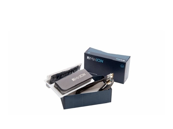
Long reads Short reads Basic Overview of Sequencing Technologies Company Platform Read Length Time per run Number of reads per unit Common error Illumina Hi. Seq 3000/4000 2 X 150 5 days ~312 million Substitution 454 Life Sciences GS FLX Titanium ≤ 1000 XL 700 Mb/day ~150, 000 indel ABI SOLi. D 5500 xl W 25 -50 5 -8 days ~300 million Substitution Pacific Biosciences Pac. Bio RS 10 kb-15 kb “short” ~50, 000 indel Oxford Nanopore Min. ION Kilobase range 2 days Tens of millions

Hi. Seq 3000/4000

How much to sequence? (read number * read length in bp) Coverage = (The number of times a site in the genome is represented by a read) Genome size in bp

How much to sequence? Say, a typical mammal… (2, 000, 000 * 150) 100 X = 3, 000, 000 My advice: go with Illumina Hi. Seq

Illumina Paired-end and Mate-pairs Paired-end (PE) “short insert library” sequencing • Genome is fragmented to desired lengths • Reads one end of the molecule, flips and then reads the other end • Generates read pairs with a known distance between them orientation FR 500 bp Mate-pair (MP)”jumping library” sequencing • Circularizes longer molecules (2 kb-25 kb) • Biotinylated, fragmented, enriched, and sequenced biotin RF

Repeats Resolved • Repeats can be resolved using paired-end information • If one end of a read is unique, then you can map both reads. • However, for longer repeats (i. e. LINEs) this will uniquenot work. repetitive • Hence Illumina-based genomes tend to be fragmented. v

Libraries Total Data (Gb) Sequence Coverage 200 bp paired-end 149. 1 51. 2 X 500 bp paired-end 141. 7 48. 7 X 3 kb mate-paired 57. 3 19. 7 X 5 kb mate-paired 72. 5 24. 9 X 10 kb mate-paired 28. 5 9. 8 X 449. 1 154. 3 X Keane et al. (2015), Cell Reports

Libraries No. reads Sequence Coverage 200 bp paired-end 1, 222, 612, 586 44 X 300 bp paired-end 1, 186, 573, 102 42 X 1 kb paired-end 468, 101, 028 17 X 2 kb mate-paired 147, 436, 368 5 X 4 kb mate-paired 182, 973, 840 6 X 10 kb mate-paired 112, 067, 096 4 X 3, 319, 764, 020 118 X 2. 9 Gb expected genome size Tollis et al. , submitted

Fastq format • Each sequence has four lines 1. 2. 3. 4. sequence name starting with “@” Nucleotide sequence Empty line except for “+” Quality score information.

Phred Quality Scores Logarithmically linked to error probabilities Phred Quality Score Probability of Error Base Call Accuracy 10 1 in 10 90% 20 1 in 100 99% 30 1 in 1, 000 99. 9% 40 1 in 10, 000 99. 99% 50 1 in 100, 000 99. 999% 60 1 in 1, 000 99. 9999%

Data Quality Control • Quality score? • GC content? • Sequence duplication levels? • Overrepresented sequences, or adaptors?

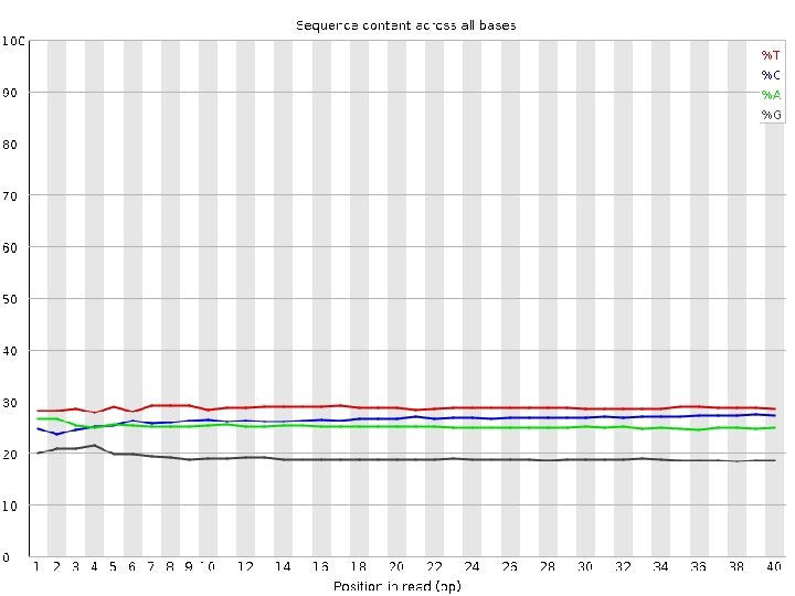
FASTQC • check quality score across the length of the reads • Good data example

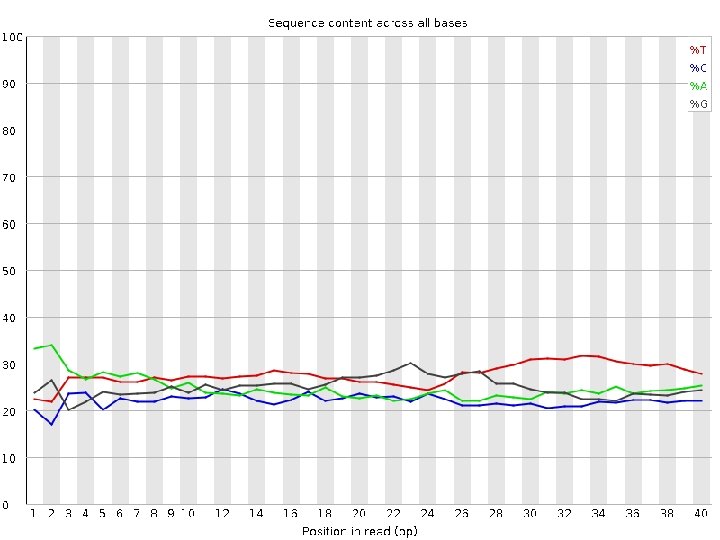
FASTQC bad data!

trimming • Trimmomatic (Bolger et al. 2014 Bioinformatics) – Paired end mode: • • • ILLUMINACLIP – trim adapters using database HEADCROP LEADING: 3 TRAILING: 3 SLIDINGWINDOW: 4: 15 MINLEN – Will trim entire dataset in pairs (F and R), and output singletons whose mates were eliminated

Three types of biases in NGS data • Systematic bias – – Problem with PCR, sequencer or library prep Errors in base-calling GC bias High duplication rates • Coverage bias • Batch effects – Non-biological differences between experimental groups

Error correction • Substitution errors are most common in Illumina datasets – In theory, errors should be infrequent (0. 0001) and random – But if you have 1 billion reads, that’s 100, 000 errors • Can be addressed by laying out all the reads covering a position • Use majority of reads to find (rare) erroneous sites, and correct them

Error correction • Error correction needs to be done before assembly! • K-spectrum-based correcting: – Reads are broken up into k-mers – Distances between k-mers are calculated – Errors are corrected • Some tools are: – SOAPdenovo error correction (Li et al. 2010) – Quake (Kelley et al. 2010) – Reptile (Yang et al. 2010)

homozygous heterozygous 27 -mer spectrum for desert tortoise (Gopherus agassizii, Tollis et al. , submitted) • Low frequency k-mers (those occurring once or twice) are likely to contain errors • Other information from k-mer frequency spectrum: • Actual coverage, given repetitiveness and heterozygosity across genome • Homozygotes should in theory be 2 X coverage of heterozygotes

Merging reads • Joins together overlapping reads to create single-end reads • If you have 180/200 bp libraries and ~100 bp reads, this is recommended. • Speeds up assembly considerably so the assembler does not have to calculate the distance between these reads. • FLASH, Cope, PEAR are some tools that do this. Forward read Read pairs merge Single end read Reverse read

Choose genome, gather info DNA Library preparation Sequencing Quality check Trimming Error correction Merge overlapping reads ASSEMBLE!

Best Assembly Advice • Remember: your goal is to have a genome assembly. • But you will not be doing one assembly. • In the end you will have many assemblies to choose from. – Because you will be doing a lot of work! • Use a lot of assembly tools for a lot of k values. – Large k can better resolve repeats – Comes at coverage cost • The whole process should take a few months.

Some Assemblers Canada’s Michael Smith Genome Sciences Centre Beijing Genomics Institute Kajitani et al. , 2014 Meraculous – Joint Genomes Institute Ma. SURCA – Maryland Genome Assembly Group

ABy. SS • Three-step process: 1. Unitig – single end assembly (no PE) 2. Contig – contigs using PE 3. Scaffolding • Optimize the parameter k by running the unitig process as an array – i. e. , every odd value between 27 and 99 – Uses MPI – For instance, run the array on 72 cpus across 6 nodes

Assembling contigs using multiple libraries in ABy. SS abyss-pe k=64 name=ecoli lib='pe 200 pe 500' pe 200='pe 200_1. fa pe 200_2. fa' pe 500='pe 500_1. fa pe 500_2. fa' se='se 1. fa se 2. fa' Library pe 200 has reads in two files, pe 200_1. fa and pe 200_2. fa. Library pe 500 has reads in two files, pe 500_1. fa and pe 500_2. fa. Single-end reads are stored in two files, se 1. fa and se 2. fa.

Scaffolding using ABy. SS abyss-pe k=64 name=ecoli lib='pe 1 pe 2' mp='mp 1 mp 2' pe 1='pe 1_1. fa pe 1_2. fa' pe 2='pe 2_1. fa pe 2_2. fa' mp 1='mp 1_1. fa mp 1_2. fa' mp 2='mp 2_1. fa mp 2_2. fa' Mate pairs are used for scaffolding, so do not add to coverage ABy. SS will estimate the true distances between reads using it’s own mapper

SOAPdenovo 2 config file max_rd_len=100 #maximal read length [LIB] avg_ins=200 #average insert size reverse_seq=0 #if sequence needs to be reversed asm_flags=3 #in which part(s) the reads are used rd_len_cutoff=100 #use only first 100 bps of each read rank=1 #in which order the reads are used while scaffolding pair_num_cutoff=3 # cutoff of pair number for a reliable connection (at least 3 for short insert size) map_len=32 #minimum aligned length to contigs for a reliable read location (at least 32 for short insert size) q 1=/path/**LIBNAMEA**/fastq 1_read_1. fq q 2=/path/**LIBNAMEA**/fastq 1_read_2. fq q=/path/**LIBNAMEA**/fastq 1_read_single. fq q=/path/**LIBNAMEA**/fastq 2_read_single. fq. . . . continued

SOAPdenovo 2 config file [LIB] avg_ins=2000 reverse_seq=1 asm_flags=2 rank=2 pair_num_cutoff=5 # cutoff of pair number for a reliable connection (at least 5 for large insert size) map_len=35 #minimum aligned length to contigs for a reliable read location (at least 35 for large insert size) q 1=/path/**LIBNAMEB**/fastq_read_1. fq q 2=/path/**LIBNAMEB**/fastq_read_2. fq

Gap closing • Every time two contigs are joined on a scaffold, a gap is created (NNN). • Reads can be mapped to the edges of gaps to close them. NNNNNN • Memory-intensive process but can reduce Ns in your genome. – Hundreds of GB RAM – A few days time • Gap Filler (Boetzer and Pirovano 2012 Genome Biology) • Gap. Closer from SOAPdenovo • Sealer (Paulino et al. 2015 BMC Bioinformatics)

1. Don’t trust the results of a single assembly. • Generate several assemblies with different assemblers and/or parameters. 2. Assemblers that work well with data from one species may not work well in another. 3. Scaffold contiguity may not be related to gene coverage. 4. Heterozygosity of target genome is a big issue. 5. Don’t place too much trust in a single metric.

Contig or Scaffold N 50 • Most widely used statistic for genome assemblies • Measure of contiguity • Take all contigs and sort them from shortest to longest. The N 50 is the length of the contig for which half of the assembly is comprised of contigs at least this length. • More informative than mean

Contig or Scaffold N 50 • 1, 1, 2, 2, 3, 4, 6, 6, 8, 9, 9, 9, 10, 24 – Mean = 5 – N 50 = 9 • N 50 can be manipulated if you eliminate small contigs – Which may be useless anyway • NG 50 – uses genome size instead of assembly length

N 50 Stats for Desert Tortoise Candidate Assemblies 120000 100000 80000 60000 N 50 40000 20000 3 k 5 P_ _k AP SO SO A 59 7 k 6 P_ SO A 3 k 8 P_ SO A P y. S AB k 8 3 S_ y. S AB S_ -> k 8 3 - SS >S PA OA CE 3 k 8 S_ y. S AB Pl at an us 0 (Tollis et al. , submitted)

Assessing Gene Space • Core Eukaryotic Genes Mapping Approach (CEGMA ) – Parra et al. (2007) – Found 458 genes highly conserved across eukaryotes in the eu. Karyotic Orthologous Groups (KOG) database – tblastn of CEGs to your genome – Refines gene models using HMMs • Proportion of 248 of the most highly conserved single-copy CEGs can be used to estimated how many genes you have in your assembly

CEG Representation Not Necessarily Related to N 50 Keith Bradnam

Benchmarking Universal Single-Copy Orthologs (BUSCO) • Similar to CEGMA • Based on Ortho. DB instead of outdated KOGs database • Clade-specific conserved single-copy orthologs – 3, 023 for vertebrates – 2, 675 for arthropods

Computed BUSCO Assessments for Vertebrate Species Human Mouse Platypus Data Type BUSCO Benchmarks Genome C: 89% [D: 1. 5%], F: 6. 0%, M: 4. 5%, n: 3023 Gene set C: 99% [D: 1. 7%], F: 0. 0%, M: 0. 0%, n: 3023 Genome C: 78% [D: 3. 0%], F: 19%, M: 2. 5%, n: 3023 Gene set C: 99% [D: 2. 5%], F: 99%, M: 0. 1%, n: 3023 Genome C: 55% [D: 0. 8%], F: 25%, M: 18%, n: 3023 Gene set C: 72% [D: 1. 1%], F: 19%, M: 8. 2%, n: 3023 BUSCO: assessing genome assembly and annotation completeness with single-copy orthologs. Felipe A. Simão, Robert M. Waterhouse, Panagiotis Ioannidis, Evgenia V. Kriventseva, and Evgeny M. Zdobnov Bioinformatics, published online June 9, 2015

Rescaffolding • SSPACE (Boetzer et al. , 2010) – – – Map reads to existing contigs/scaffolds with bowtie Position and orientation of each mapped pair is stored in hash Read pairs across contigs are joined Done iteratively using libraries of increasing size RAM-intensive • Can do this using different contigs/scaffolds from different assemblers to try to improve contiguity • Best with new data (mate pairs or long reads) • ABy. SS and SOAPdenovo 2 have standalone scaffolders too

RNA Scaffolding • Nice alternative if you have RNA-Seq data for your genome project (i. e. , for annotation) • Genes may be split across separate scaffolds due to long introns containing repeats. • Assemble transcriptome, model ORFs and collect those which have BLAST hits, BLAT genes to assembly • Join scaffolds which map to the same gene. • L_RNA_scaffolder (Xue et al. 2013 BMC Genomics)

RNA Scaffolding Tollis et al. , submitted

Dovetail Genomics • • Chicago Library method – reconstituted chromatin Vast insert sizes Sequence the libraries at ~95 X coverage Used to rescaffold Illumina assemblies

Choose genome, gather info ASSEMBLE! DNA Library preparation Assemble again and again (different tools, kmers) Sequencing Fill gaps Quality check Evaluate assembly contiguity Trimming Evaluate assembly gene content Error correction Choose a final assembly Merge overlapping reads Re-scaffold ASSEMBLE! ANNOTATE!

http: //weatherby. genetics. utah. edu/MAKER/wiki/index. php/MAKER_Tutorial

Repeat Masking • Essential step before annotation • Many repeats contain ORFs, can be mistaken as genes. • Repeats should be “masked” before you try to annotate genes – “NNNNN” = hardmasked – “atcg” = softmasked • Better for downstream BLAST or genome alignment

Two Methods of Repeat Finding • Database method – Repeat. Masker (repeatmasker. org) • Blast Rep. Base elements to your genome • Good for mammals or model organisms • Ascertainment bias – species have unique repeats – Human: 50% masked with “homo sapiens” repeats. – Humpack whale: 38% masked with “mammalia” repeats. – Glass lizard: 13% masked with “vertebrate” repeats

Two Methods of Repeat Finding • De novo method – Repeat. Modeler (repeatmasker. org) • • Blast your genome to itself Models repeats without a priori knowledge Good for finding species-specific repeats May miss low-copy number repeats • I find best results in a three-pronged approach: 1. 2. 3. Run Repeat. Masker on the genome using clade-appropriate Rep. Base library. Run Repeat. Modeler on the unmasked remainder of the genome. Combine the Rep. Base library with the de novo library and run Repeat. Masker again

Gene Annotation Raw Materials • Ab-initio gene prediction software – SNAP – Augustus – Requires training to your specific species • Protein homology – NCBI, Ensembl, Uni. Prot/Swiss. Prot • Expression data – RNA-Seq – This is the only direct evidence used

MAKER (Holt and Yandell, 2011) http: //weatherby. genetics. utah. edu/MAKER/wiki/index. php/MAKER_Tutorial

Conclusion • Post-assembly and post-annotation is where the science begins. – Differential expression experiments? • You’re going to need more data (RNA-seq) – Population genomics? • You’re going to need more data (whole genome) • Was that so hard? • Get out there and assemble.

Thank You ASU School of Life Sciences Kenro Kusumi, Ph. D. Melissa Wilson-Sayres, Ph. D. ASU_genomics group Biodesign Institute Carlo Maley, Ph. D. Marc. tollis@asu. edu