DAY 9 EXCEL CHAPTER 6 RAHUL KAVI Rahul

DAY 9: EXCEL CHAPTER 6 RAHUL KAVI Rahul. Kavi@mail. wvu. edu September 17, 2013 1

LAST CLASS • • • Freezing Rows and Columns Tables Sorting Filtering Total Row Conditional Formatting 2

OUTLINES/GROUPS • Groups allow you to hide raw data while you work with the calculations derived from that data • You can group rows or columns • Easily hide and unhide large chunks of data • Data->Group 3

GROUP SUBTOTALS • Allows you to aggregate groups of data using one of several functions – Sum – Average – Variance – Standard Deviation – Min/Max – Count 4

USING GROUP SUBTOTALS • • Sort the data by the group identifier Does not work on tables Data->Subtotal Select the sorted column for “At each change in: ” • Select your aggregation function • Select which columns to subtotal 5

PIVOT TABLES • Insert->Pivot. Table • Ensure the range is correct • Select target location (new worksheet or existing worksheet) 6

ADDING COLUMNS • Click check mark to add column • Automatically aggregates with SUM(), but you can choose a different function 7

ADJUSTING GROUPING • Move the section number from the “Values” area to the “Row Labels” area • Move “Section” above “Student” to group by sections • Values can be rearranged to adjust the column order 8

UPDATING PIVOT TABLES • Pivot. Tables do not automatically update if you change the source data • You can force a refresh via Pivot. Table Tools->Options->Refresh 9

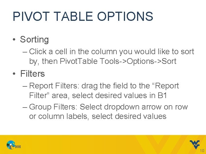
PIVOT TABLE OPTIONS • Sorting – Click a cell in the column you would like to sort by, then Pivot. Table Tools->Options->Sort • Filters – Report Filters: drag the field to the “Report Filter” area, select desired values in B 1 – Group Filters: Select dropdown arrow on row or column labels, select desired values 10

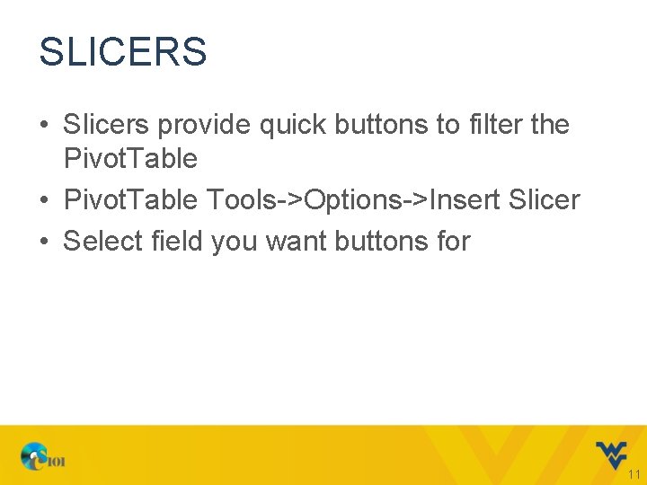
SLICERS • Slicers provide quick buttons to filter the Pivot. Table • Pivot. Table Tools->Options->Insert Slicer • Select field you want buttons for 11

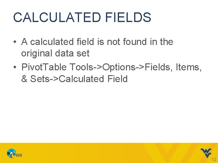
CALCULATED FIELDS • A calculated field is not found in the original data set • Pivot. Table Tools->Options->Fields, Items, & Sets->Calculated Field 12

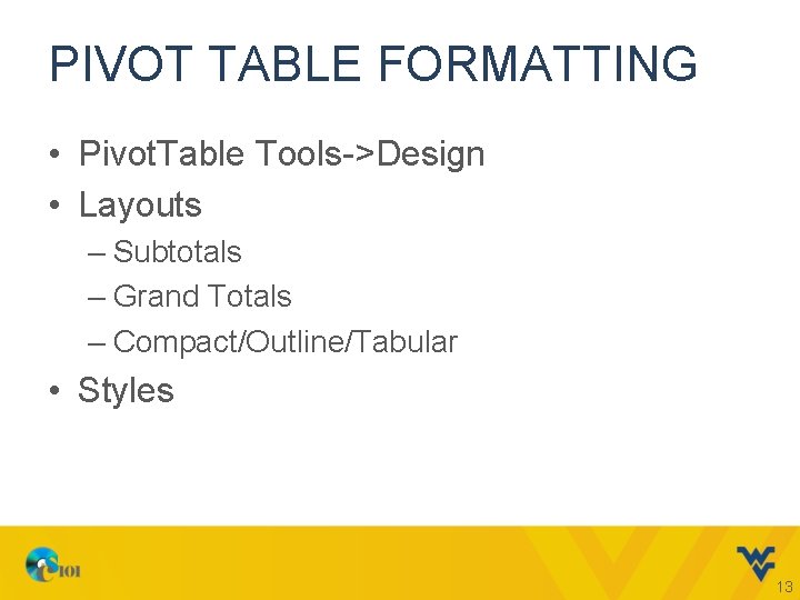
PIVOT TABLE FORMATTING • Pivot. Table Tools->Design • Layouts – Subtotals – Grand Totals – Compact/Outline/Tabular • Styles 13

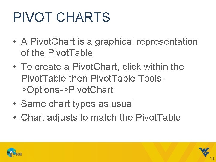
PIVOT CHARTS • A Pivot. Chart is a graphical representation of the Pivot. Table • To create a Pivot. Chart, click within the Pivot. Table then Pivot. Table Tools>Options->Pivot. Chart • Same chart types as usual • Chart adjusts to match the Pivot. Table 14

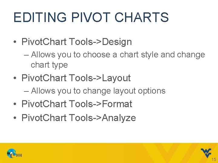
EDITING PIVOT CHARTS • Pivot. Chart Tools->Design – Allows you to choose a chart style and change chart type • Pivot. Chart Tools->Layout – Allows you to change layout options • Pivot. Chart Tools->Format • Pivot. Chart Tools->Analyze 15

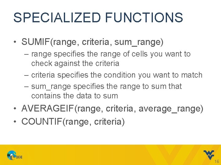
SPECIALIZED FUNCTIONS • SUMIF(range, criteria, sum_range) – range specifies the range of cells you want to check against the criteria – criteria specifies the condition you want to match – sum_range specifies the range to sum that contains the data to sum • AVERAGEIF(range, criteria, average_range) • COUNTIF(range, criteria) 16

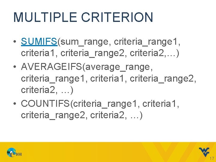
MULTIPLE CRITERION • SUMIFS(sum_range, criteria_range 1, criteria_range 2, criteria 2, …) • AVERAGEIFS(average_range, criteria_range 1, criteria_range 2, criteria 2, …) • COUNTIFS(criteria_range 1, criteria_range 2, criteria 2, …) 17

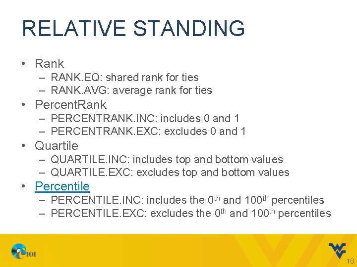
RELATIVE STANDING • Rank – RANK. EQ: shared rank for ties – RANK. AVG: average rank for ties • Percent. Rank – PERCENTRANK. INC: includes 0 and 1 – PERCENTRANK. EXC: excludes 0 and 1 • Quartile – QUARTILE. INC: includes top and bottom values – QUARTILE. EXC: excludes top and bottom values • Percentile – PERCENTILE. INC: includes the 0 th and 100 th percentiles – PERCENTILE. EXC: excludes the 0 th and 100 th percentiles 18

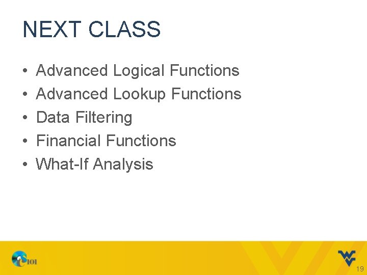
NEXT CLASS • • • Advanced Logical Functions Advanced Lookup Functions Data Filtering Financial Functions What-If Analysis 19