Datorntverk A lektion 3 Kapitel 3 Fysiska signaler

Datornätverk A – lektion 3 • Kapitel 3: Fysiska signaler. • Kapitel 4: Digital transmission.

PART II Physical Layer

Chapter 3 Signals

Figure 3. 1 Comparison of analog and digital signals

Note: Signals can be analog or digital. Analog signals can have an infinite number of values in a range; digital signals can have only a limited number of values.

Sinusvågor Periodtid T = t 2 - t 1. Enhet: s. Frekvens f = 1/T. Enhet: 1/s=Hz. T=1/f. Amplitud eller toppvärde Û. Enhet: Volt. Fasläge: θ = 0 i ovanstående exempel. Enhet: Grader eller radianer. Momentan spänning: u(t)= Ûsin(2πft+θ)

Figure 3. 4 Period and frequency

Tabell 3. 1 Enheter för periodtid och frekvens Enhet Sekunder (s) Ekvivalent 1 s Enhet Hertz (Hz) Ekvivalent 1 Hz Millisekunder (ms) 10– 3 s Kilohertz (k. Hz) 103 Hz Mikrosekunder (μs) 10– 6 s Megahertz (MHz) 106 Hz Nanosekunder (ns) 10– 9 s Gigahertz (GHz) 109 Hz Pikosekunder (ps) 10– 12 s Terahertz (THz) 1012 Hz Exempel: En sinusvåg med periodtid 1 ns har frekvens 1 GHz.

Exempel 1 Vilken frekvens i k. Hz har en sinusvåg med periodtid 100 ms? Solution Alternativ 1: Gör om till grundenheten. 100 ms = 0. 1 s f = 1/0. 1 Hz = 10/1000 k. Hz = 0. 01 k. Hz Alternativ 2: Utnyttja att 1 ms motsvarar 1 k. Hz. f = 1/100 ms = 0. 01 k. Hz.

Figure 3. 5 Relationships between different phases

Example 2 A sine wave is offset one-sixth of a cycle with respect to time zero. What is its phase in degrees and radians? Solution We know that one complete cycle is 360 degrees. Therefore, 1/6 cycle is (1/6) 360 = 60 degrees = 60 x 2 p /360 rad = 1. 046 rad

Figure 3. 6 Sine wave examples

Figure 3. 6 Sine wave examples (continued)

Figure 3. 6 Sine wave examples (continued)

Figure 3. 7 Time and frequency domains (continued)

Figure 3. 7 Time and frequency domains

Figure 3. 8 Square wave

Figure 3. 9 Three harmonics

Figure 3. 10 Adding first three harmonics

Figure 3. 11 Frequency spectrum comparison

Figure 3. 12 Signal corruption

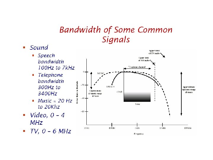
Figure 3. 13 Bandwidth

Example 3 If a periodic signal is decomposed into five sine waves with frequencies of 100, 300, 500, 700, and 900 Hz, what is the bandwidth? Draw the spectrum, assuming all components have a maximum amplitude of 10 V. Solution B = fh - fl = 900 - 100 = 800 Hz The spectrum has only five spikes, at 100, 300, 500, 700, and 900 (see Figure 13. 4 )

Figure 3. 14 Example 3

Example 5 A signal has a spectrum with frequencies between 1000 and 2000 Hz (bandwidth of 1000 Hz). A medium can pass frequencies from 3000 to 4000 Hz (a bandwidth of 1000 Hz). Can this signal faithfully pass through this medium? Solution The answer is definitely no. Although the signal can have the same bandwidth (1000 Hz), the range does not overlap. The medium can only pass the frequencies between 3000 and 4000 Hz; the signal is totally lost.

Figure 3. 16 A digital signal

Example 6 A digital signal has a bit rate of 2000 bps. What is the duration of each bit (bit interval) Solution The bit interval is the inverse of the bit rate. Bit interval = 1/ 2000 s = 0. 000500 x 106 ms = 500 ms

Figure 3. 17 Bit rate and bit interval

Figure 3. 18 Digital versus analog

Note: A digital signal is a composite signal with an infinite bandwidth.

Table 3. 12 Bandwidth Requirement Bit Rate Harmonic 1 Harmonics 1, 3, 5, 7 1 Kbps 500 Hz 2 KHz 4. 5 KHz 8 KHz 10 Kbps 5 KHz 20 KHz 45 KHz 80 KHz 100 Kbps 50 KHz 200 KHz 450 KHz 800 KHz

Note: The bit rate and the bandwidth are proportional to each other.

Figure 3. 19 Low-pass and band-pass

Note: The analog bandwidth of a medium is expressed in hertz; the digital bandwidth, in bits per second.

Note: Digital transmission needs a low-pass channel.

Note: Analog transmission can use a bandpass channel.

Figure 3. 20 Impairment types

Figure 3. 21 Attenuation

Förstärkning mätt i decibel (d. B) 1 gång effektförstärkning = 0 d. B. 2 ggr effektförstärkning = 3 d. B. 10 ggr effektförstärkning = 10 d. B. 100 ggr effektförstärkning = 20 d. B. 1000 ggr effektförstärkning = 30 d. B. Osv.

Dämpning mätt i decibel • Dämpning 100 ggr = Dämpning 20 d. B = förstärkning 0. 01 ggr = förstärkning med – 20 d. B. • Dämpning 1000 ggr = 30 d. B dämpning = -30 d. B förstärkning. • En halvering av signalen = dämpning med 3 d. B = förstärkning med -3 d. B.

Signal-brus-förhållande • Ett signal-brus-förhållande på 100 d. B innebär att den starkaste signalen är 100 d. B starkare än bruset. • Ljud som är svagare än bruset hörs inte utan dränks i bruset. • Ljudets dynamik skillnaden mellan den starkaste ljudet och det svagaste ljudet som man kan höra, och är vanligen ungefär detsamma som signal-brus-förhållandet.

Example 12 Imagine a signal travels through a transmission medium and its power is reduced to half. This means that P 2 = 1/2 P 1. In this case, the attenuation (loss of power) can be calculated as Solution 10 log 10 (P 2/P 1) = 10 log 10 (0. 5 P 1/P 1) = 10 log 10 (0. 5) = 10(– 0. 3) = – 3 d. B

Example 13 Imagine a signal travels through an amplifier and its power is increased ten times. This means that P 2 = 10∙P 1. In this case, the amplification (gain of power) can be calculated as 10 log 10 (P 2/P 1) = 10 log 10 (10 P 1/P 1) = 10 log 10 (10) = 10 (1) = 10 d. B

Example 14 One reason that engineers use the decibel to measure the changes in the strength of a signal is that decibel numbers can be added (or subtracted) when we are talking about several points instead of just two (cascading). In Figure 3. 22 a signal travels a long distance from point 1 to point 4. The signal is attenuated by the time it reaches point 2. Between points 2 and 3, the signal is amplified. Again, between points 3 and 4, the signal is attenuated. We can find the resultant decibel for the signal just by adding the decibel measurements between each set of points.

Figure 3. 22 Example 14 d. B = – 3 + 7 – 3 = +1

Figure 3. 23 Distortion

Figure 3. 24 Noise

Throughput (Genomströmningshastighet)

Figure 3. 26 Propagation time (Utbredningstid)

Chapter 4 Digital Transmission

Figure 4. 2 Signal level versus data level

Figure 4. 3 DC component

Example 1 A signal has two data levels with a pulse duration of 1 ms. We calculate the pulse rate and bit rate as follows: Pulse Rate = 1/ 10 -3= 1000 pulses/s Bit Rate = Pulse Rate x log 2 L = 1000 x log 2 2 = 1000 bps

Example 2 A signal has four data levels with a pulse duration of 1 ms. We calculate the pulse rate and bit rate as follows: Pulse Rate = = 1000 pulses/s Bit Rate = Pulse. Rate x log 2 L = 1000 x log 2 4 = 2000 bps

Figure 4. 4 Lack of synchronization

Example 3 In a digital transmission, the receiver clock is 0. 1 percent faster than the sender clock. How many extra bits per second does the receiver receive if the data rate is 1 Kbps? How many if the data rate is 1 Mbps? Solution At 1 Kbps: 1000 bits sent 1001 bits received 1 extra bps At 1 Mbps: 1, 000 bits sent 1, 000 bits received 1000 extra bps

Figure 4. 5 Line coding schemes

Note: Unipolar encoding uses only one voltage level.

Figure 4. 6 Unipolar encoding

Note: Polar encoding uses two voltage levels (positive and negative).

Figure 4. 7 Types of polar encoding

Note: In NRZ-L the level of the signal is dependent upon the state of the bit.

Note: In NRZ-I the signal is inverted if a 1 is encountered.

Figure 4. 8 NRZ-L and NRZ-I encoding

Figure 4. 9 RZ encoding

Note: A good encoded digital signal must contain a provision for synchronization.

Figure 4. 10 Manchester encoding

Note: In Manchester encoding, the transition at the middle of the bit is used for both synchronization and bit representation.

Figure 4. 11 Differential Manchester encoding

Note: In differential Manchester encoding, the transition at the middle of the bit is used only for synchronization. The bit representation is defined by the inversion or noninversion at the beginning of the bit.

Note: In bipolar encoding, we use three levels: positive, zero, and negative.

Figure 4. 12 Bipolar AMI encoding

4. 3 Sampling Pulse Amplitude Modulation Pulse Code Modulation Sampling Rate: Nyquist Theorem How Many Bits per Sample? Bit Rate

PCM = Pulse Code Modulation = Digitalisering av analoga signaler och seriell överföring Sifferexempel från PSTN = publika telefonnätet: 011011010001. . . 1 0 Antivikningsfilter Sampler AD-omvandlare med seriell utsignal DAomvandlare Interpolationsfilter Högtalare Mikrofon 34004000 Hz filter 8000 sampels per sek 8 bit per sampel dvs 64000 bps per tfnsamtal 28 = 256 spänningsnivåer

Exempel En 6 sekunder lång ljudinspelning digitaliseras. Hur stor är inspelningens informationsmängd? a) 22000 sampels/sekund, 256 kvantiseringsnivåer. 22000 sampels * 6 s * 8 bit = 1056000 bit. b) 22000 sampels/sekund, 16 kvantiseringsnivåer. 22000 sampels * 6 s * 4 bit = 528000 bit. c) 5500 sampels/sekund, 256 kvantiseringsnivåer. 5500 sampels * 6 s * 8 bit = 264000 bit.

Samplingsteoremet • • • f < fs/2 Den högsta frekvens som kan samplas är halva samplingsfrekvensen. Om man samplar högre frekvens än fs/2 så byter signalen frekvens, dvs det uppstår vikningsdistorsion (aliasing). För att undvika vikningsdistorsion så har man ett anti-vikningsfilter innan samplingen, som tar bort frekvenser över halva samplingsfrekvensen. Interpolationsfiltret används vid rekonstruktion av den digitala signalen för att ”gissa” värden mellan samplen. Ett ideal interpolationsfilter skulle kunna återskapa den samplade signalen perfekt om den uppfyller samplingsteoremet. I verkligheten finns inga ideala filter. Följdregel: Nyqvist’s sats säger att max datahastighet = 2 B 2 log M, där M är antal nivåer, och B är signalens bandbredd, oftast lika med signalens övre gränsfrekvens.

Figure 4. 18 PAM

Note: Pulse amplitude modulation has some applications, but it is not used by itself in data communication. However, it is the first step in another very popular conversion method called pulse code modulation.

Figure 4. 19 Quantized PAM signal

Figure 4. 20 Quantizing by using sign and magnitude

Note: According to the Nyquist theorem, the sampling rate must be at least 2 times the highest frequency.

Example 4 What sampling rate is needed for a signal with a bandwidth of 10, 000 Hz (1000 to 11, 000 Hz)? Solution The sampling rate must be twice the highest frequency in the signal: Sampling rate = 2 x (11, 000) = 22, 000 samples/s

Example 5 A signal is sampled. Each sample requires at least 12 levels of precision (+0 to +5 and -0 to -5). How many bits should be sent for each sample? Solution We need 4 bits; 1 bit for the sign and 3 bits for the value. A 3 -bit value can represent 23 = 8 levels (000 to 111), which is more than what we need. A 2 -bit value is not enough since 22 = 4. A 4 -bit value is too much because 24 = 16.

Example 6 We want to digitize the human voice. What is the bit rate, assuming 8 bits per sample? Solution The human voice normally contains frequencies from 0 to 4000 Hz. Sampling rate = 4000 x 2 = 8000 samples/s Bit rate = sampling rate x number of bits per sample = 8000 x 8 = 64, 000 bps = 64 Kbps

Distorsion till följd av digitalisering • Vikningsdistorsion ○ Inträffar om man inte filtrerar bort frekvenser som är högre än halva samplingsfrekvensen. • Kvantiseringsdistorsion (kvantiseringsbrus) ○ Avrundningsfelet låter ofta som ett brus. ○ Varje extra bit upplösning ger dubbelt så många spänningsnivåer, vilket ger en minskning av kvantiseringsdistorsionen med 6 d. B. 16 bit upplösning ger ett signal-brus-förhållande på ca 16*6 = 96 d. B (beroende på hur man mäter detta förhållande. ) ○ Svaga ljud avrundas bort, eller dränks i kvantiseringsbruset.