DataParallel Programming using Sa C lecture 2 F

Data-Parallel Programming using Sa. C lecture 2 F 21 DP Distributed and Parallel Technology Sven-Bodo Scholz

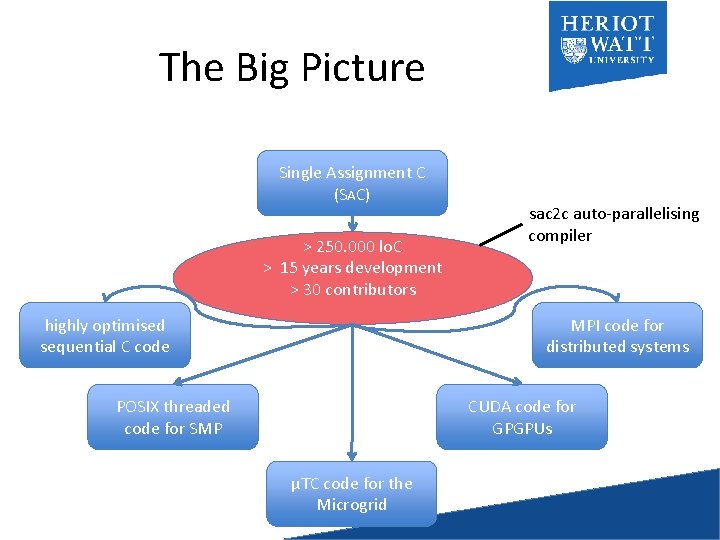
The Big Picture Single Assignment C (SAC) > 250. 000 lo. C > 15 years development > 30 contributors highly optimised sequential C code sac 2 c auto-parallelising compiler MPI code for distributed systems POSIX threaded code for SMP CUDA code for GPGPUs μTC code for the Microgrid

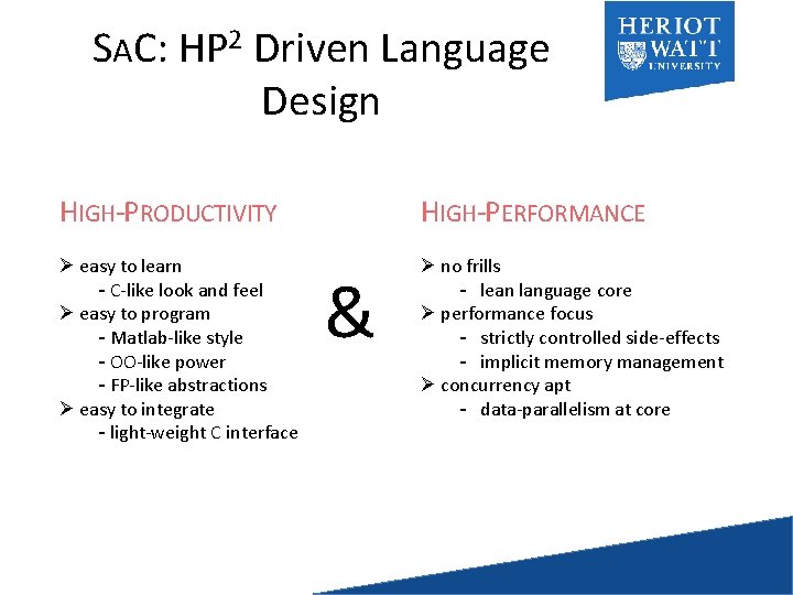
SAC: HP 2 Driven Language Design HIGH-PRODUCTIVITY HIGH-PERFORMANCE Ø easy to learn - C-like look and feel Ø easy to program - Matlab-like style - OO-like power - FP-like abstractions Ø easy to integrate - light-weight C interface Ø no frills - lean language core Ø performance focus - strictly controlled side-effects - implicit memory management Ø concurrency apt - data-parallelism at core &

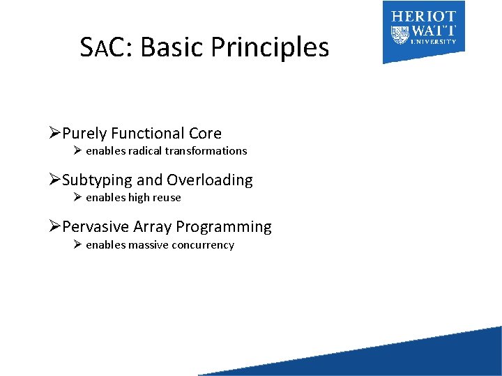
SAC: Basic Principles ØPurely Functional Core Ø enables radical transformations ØSubtyping and Overloading Ø enables high reuse ØPervasive Array Programming Ø enables massive concurrency

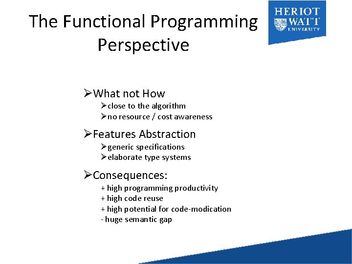
The Functional Programming Perspective ØWhat not How Øclose to the algorithm Øno resource / cost awareness ØFeatures Abstraction Øgeneric specifications Øelaborate type systems ØConsequences: + high programming productivity + high code reuse + high potential for code-modication - huge semantic gap

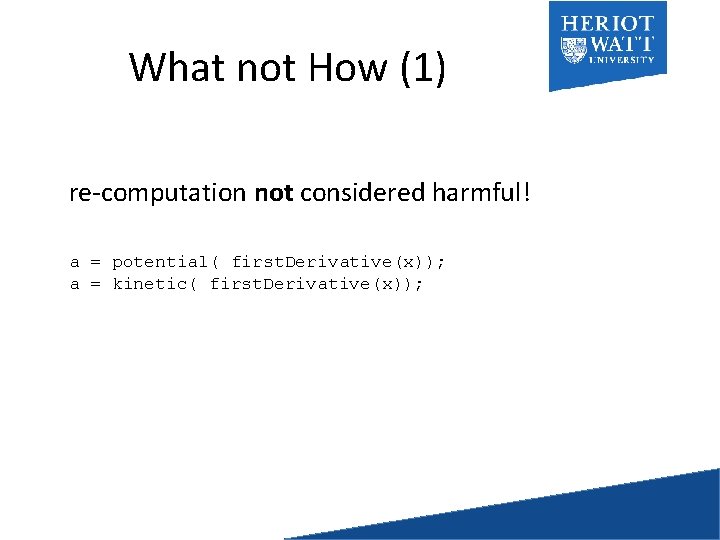
What not How (1) re-computation not considered harmful! a = potential( first. Derivative(x)); a = kinetic( first. Derivative(x));

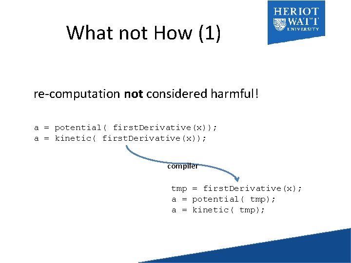
What not How (1) re-computation not considered harmful! a = potential( first. Derivative(x)); a = kinetic( first. Derivative(x)); compiler tmp = first. Derivative(x); a = potential( tmp); a = kinetic( tmp);

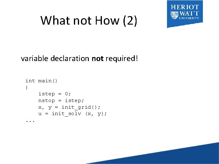
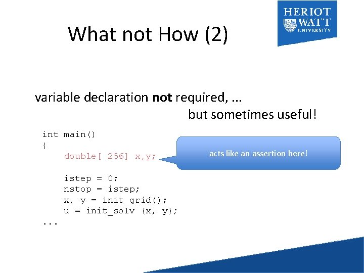
What not How (2) variable declaration not required! int main() { istep = 0; nstop = istep; x, y = init_grid(); u = init_solv (x, y); . . .

What not How (2) variable declaration not required, . . . but sometimes useful! int main() { double[ 256] x, y; istep = 0; nstop = istep; x, y = init_grid(); u = init_solv (x, y); . . . acts like an assertion here!

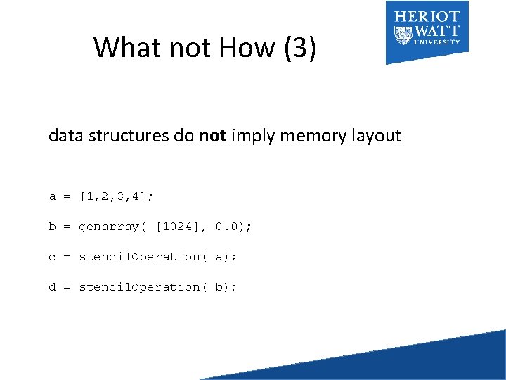
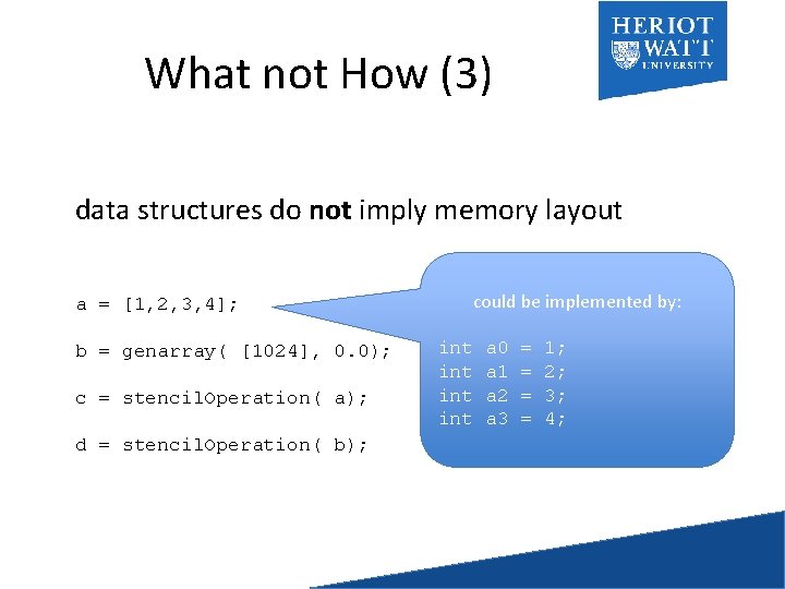
What not How (3) data structures do not imply memory layout a = [1, 2, 3, 4]; b = genarray( [1024], 0. 0); c = stencil. Operation( a); d = stencil. Operation( b);

What not How (3) data structures do not imply memory layout a = [1, 2, 3, 4]; b = genarray( [1024], 0. 0); c = stencil. Operation( a); d = stencil. Operation( b); could be implemented by: int int a 0 a 1 a 2 a 3 = = 1; 2; 3; 4;

What not How (3) data structures do not imply memory layout a = [1, 2, 3, 4]; b = genarray( [1024], 0. 0); c = stencil. Operation( a); d = stencil. Operation( b); or by: int a[4] = {1, 2, 3, 4};

What not How (3) data structures do not imply memory layout or by: a = [1, 2, 3, 4]; b = genarray( [1024], 0. 0); c = stencil. Operation( a); d = stencil. Operation( b); adesc_t a = malloc(. . . ) a->data[0] = 1; a->desc[1] = 2; a->desc[2] = 3; a->desc[3] = 4;

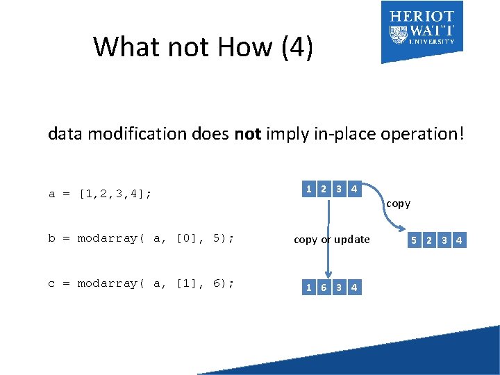
What not How (4) data modification does not imply in-place operation! a = [1, 2, 3, 4]; 1 2 3 4 b = modarray( a, [0], 5); copy or update c = modarray( a, [1], 6); 1 6 3 4 copy 5 2 3 4

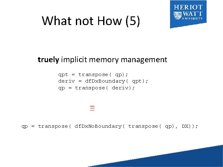
What not How (5) truely implicit memory management qpt = transpose( qp); deriv = df. Dx. Boundary( qpt); qp = transpose( deriv); ≡ qp = transpose( df. Dx. No. Boundary( transpose( qp), DX));

Subtyping and Overloading ØAims Øextreme code reuse Ømulti-inheritance ØConsequences: + high programming productivity + high code reuse - huge semantic gap

Subtyping in Sa. C int[*] a; int[. , . ] m; int[1, 0] m 2; a = [[1, 2], [3, 4]]; m = [[]]; m 2 = [[]];

Function Overloading double method. X( double[. , . ] a, double[*] b) {. . . } double method. X( double[2, 2] a, double[. , . ] b) {. . . } double method. X( double[. , . ] a, double b) {. . . }

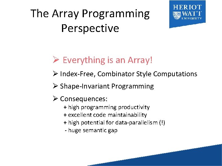
The Array Programming Perspective Ø Everything is an Array! Ø Index-Free, Combinator Style Computations Ø Shape-Invariant Programming Ø Consequences: + high programming productivity + excellent code maintainability + high potential for data-parallelism (!) - huge semantic gap

Basic Operations dim(42) == 0 dim( [1, 2, 3]) == 1 dim([[1, 2, 3], [4, 5, 6]] ) == 2 shape( 42) == [] shape( [1, 2, 3]) == [3] shape( [[1, 2, 3], [4, 5, 6]] ) == [2, 3] a = [[1, 2, 3], [4, 5, 6]]; a[[1, 0]] == 4 a[[1]] == [1, 5, 6] a[[]] == a 19

The Usual Suspects a = [1, 2, 3]; b = [4, 4, 2]; a+b == [5, 6, 5]; a<=b == [true, false]; sum(a) == 6. . . 20

Matlab/ APL stuff a = [[1, 2, 3], [4, 5, 6]]; take( [2, 1], a) == [[1], [4]] take( [1], a) == [[1, 2, 3]] != [1, 2, 3] take( [], a) == a take( [-1, 2], a) == [[4, 5]]. . . 21

Set Notation { iv -> a[iv] + 1 } == a + 1 { [i, j] -> mat[[j, i]] } == transpose( mat) { [i, j]->(i==j? mat[[i, j]]: 0)} 22

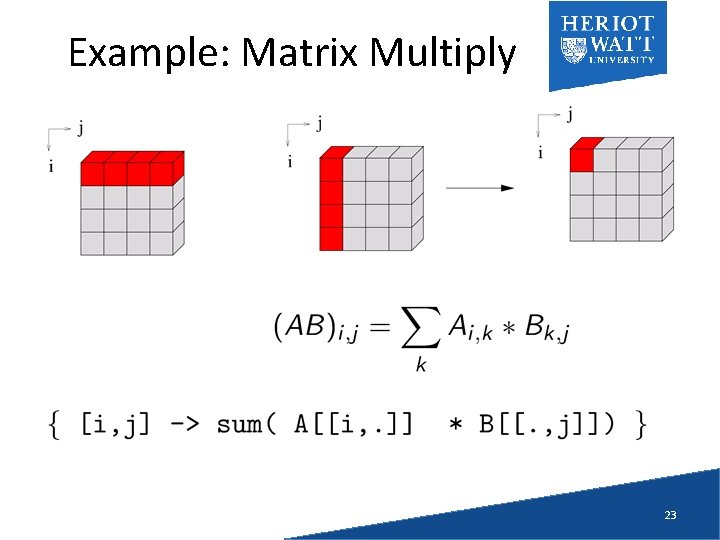
Example: Matrix Multiply 23

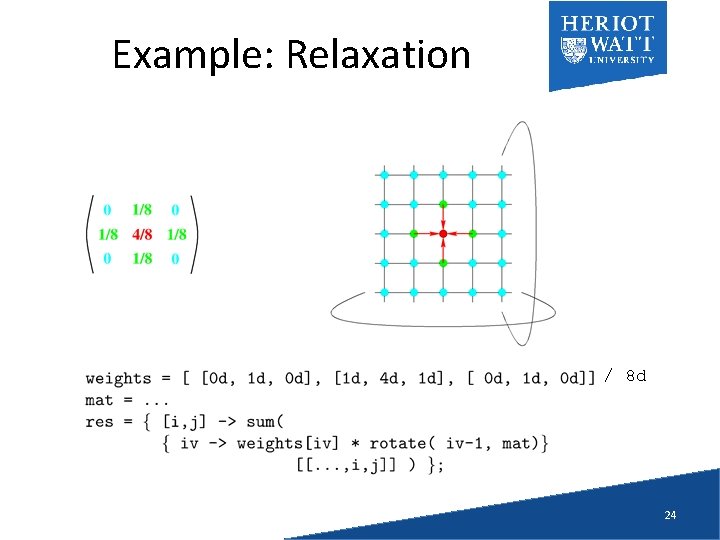
Example: Relaxation / 8 d 24

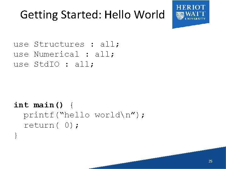
Getting Started: Hello World use Structures : all; use Numerical : all; use Std. IO : all; int main() { printf(“hello worldn”); return( 0); } 25

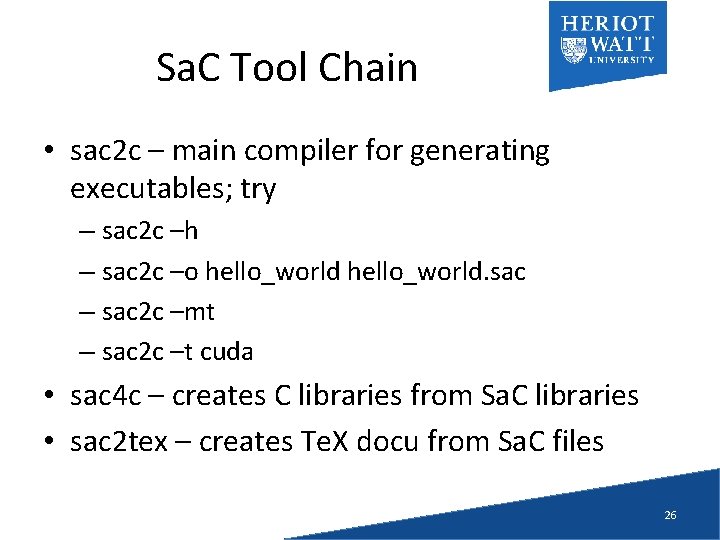
Sa. C Tool Chain • sac 2 c – main compiler for generating executables; try – sac 2 c –h – sac 2 c –o hello_world. sac – sac 2 c –mt – sac 2 c –t cuda • sac 4 c – creates C libraries from Sa. C libraries • sac 2 tex – creates Te. X docu from Sa. C files 26