DataIntensive Distributed Computing CS 431631 451651 Winter 2019
 Part 4: Analyzing Graphs (1/2) February")
Data-Intensive Distributed Computing CS 431/631 451/651 (Winter 2019) Part 4: Analyzing Graphs (1/2) February 5, 2019 Adam Roegiest Kira Systems These slides are available at http: //roegiest. com/bigdata-2019 w/ This work is licensed under a Creative Commons Attribution-Noncommercial-Share Alike 3. 0 United States See http: //creativecommons. org/licenses/by-nc-sa/3. 0/us/ for details

Data Mining Analyzing Relational Data Analyzing Graphs Analyzing Text Structure of the Course “Core” framework features and algorithm design
, where V represents the set of vertices")
What’s a graph? G = (V, E), where V represents the set of vertices (nodes) E represents the set of edges (links) Edges may be directed or undirected Both vertices and edges may contain additional information outlinks edges (links) outgoing (outbound) edges out-degree vertex (node) edges (links) in-degree inlinks incoming (inbound) edges “incident”

Examples of Graphs Hyperlink structure of the web Physical structure of computers on the Internet Interstate highway system Social networks We’re mostly interested in sparse graphs!
")
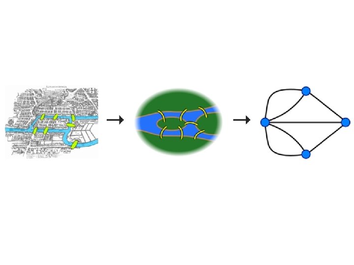
Source: Wikipedia (Königsberg)
")
Source: Wikipedia (Kaliningrad)

Some Graph Problems Finding shortest paths Routing Internet traffic and UPS trucks Finding minimum spanning trees Telco laying down fiber Finding max flow Airline scheduling Identify “special” nodes and communities Halting the spread of avian flu Bipartite matching match. com Web ranking Page. Rank

What makes graphs hard? Irregular structure Fun with data structures! Irregular data access patterns Fun with architectures! Iterations Fun with optimizations!
 A large class of graph algorithms involve: Local")
Graphs and Map. Reduce (and Spark) A large class of graph algorithms involve: Local computations at each node Propagating results: “traversing” the graph Key questions: How do you represent graph data in Map. Reduce (and Spark)? How do you traverse a graph in Map. Reduce (and Spark)?

Representing Graphs Adjacency matrices Adjacency lists Edge lists

Adjacency Matrices Represent a graph as an n x n square matrix M n = |V| Mij = 1 iff an edge from vertex i to j 1 1 0 2 1 3 0 4 1 2 1 0 1 1 3 4 1 1 0 0 0 1 0 0 2 1 3 4

Adjacency Matrices: Critique Advantages Amenable to mathematical manipulation Intuitive iteration over rows and columns Disadvantages Lots of wasted space (for sparse matrices) Easy to write, hard to compute

Adjacency Lists Take adjacency matrix… and throw away all the zeros 1 1 0 2 1 3 0 4 1 2 1 0 1 1 3 4 1 1 0 0 0 1: 2, 4 2: 1, 3, 4 3: 1 4: 1, 3 we e v a h e her w , t i a W re? o f e b s i seen th
 Easy to compute over outlinks")
Adjacency Lists: Critique Advantages Much more compact representation (compress!) Easy to compute over outlinks Disadvantages Difficult to compute over inlinks

Edge Lists Explicitly enumerate all edges 1 1 0 2 1 3 0 4 1 2 1 0 1 1 3 4 1 1 0 0 0 1 0 0 (1, 2) (1, 4) (2, 1) (2, 3) (2, 4) (3, 1) (4, 3)

Edge Lists: Critique Advantages Easily support edge insertions Disadvantages Wastes spaces
 … …")
Graph Partitioning Vertex Partitioning Edge Partitioning (A lot more detail later…) … …

Storing Undirected Graphs Standard Tricks 1. Store both edges Make sure your algorithm de-dups 2. Store one edge, e. g. , (x, y) st. x < y Make sure your algorithm handles the asymmetry

Basic Graph Manipulations Invert the graph flat. Map and regroup Adjacency lists to edge lists flat. Map adjacency lists to emit tuples Edge lists to adjacency lists group. By Framework does all the heavy lifting!

Co-occurrence of characters in Les Misérables Source: http: //bost. ocks. org/mike/miserables/

Co-occurrence of characters in Les Misérables Source: http: //bost. ocks. org/mike/miserables/

Co-occurrence of characters in Les Misérables ? ated r e n e g his t e k i l s ion t a z i l a u s s? i n v o i e t r a a t i Lim How Source: http: //bost. ocks. org/mike/miserables/

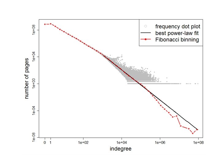
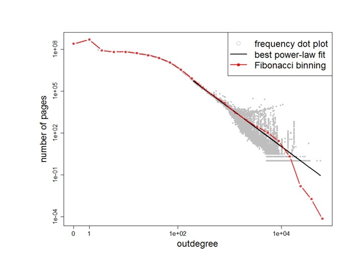
What does the web look like? Analysis of a large webgraph from the common crawl: 3. 5 billion pages, 129 billion links Meusel et al. Graph Structure in the Web — Revisited. WWW 2014.
 – revisited")
Broder’s Bowtie (2000) – revisited

What does the web look like? Very roughly, a scale-free network Fraction of k nodes having k connections: (i. e. , degree distribution follows a power law)
 “Power laws,")
a L r we Po Figure from: Newman, M. E. J. (2005) “Power laws, Pareto distributions and Zipf's law. ” Contemporary Physics 46: 323– 351. e r a ws w y r eve ! e r he

k? o o ceb a F t ou b a t Figure from: Seth A. Myers, Aneesh Sharma, Pankaj Gupta, and Jimmy Lin. Information Network or Social Network? The Structure of the Twitter Follow Graph. WWW 2014. Wha

What does the web look like? Very roughly, a scale-free network Other Examples: Internet domain routers Co-author network Citation network Movie-Actor network ? y h W
 Preferential Attachment Also: Matthew")
(In this installment of “learn fancy terms for simple ideas”) Preferential Attachment Also: Matthew Effect For unto every one that hath shall be given, and he shall have abundance: but from him that hath not shall be taken even that which he hath. — Matthew 25: 29, King James Version.

BTW, how do we compute these graphs?

Count. Source: http: //www. flickr. com/photos/guvnah/7861418602/

BTW, how do we extract the webgraph? The webgraph… is big? ! A few tricks: Integerize vertices (montone minimal perfect hashing) Sort URLs Integer compression ! B G 58 webgraph from the common crawl: 3. 5 billion pages, 129 billion links Meusel et al. Graph Structure in the Web — Revisited. WWW 2014.
 A large class of graph algorithms involve: Local")
Graphs and Map. Reduce (and Spark) A large class of graph algorithms involve: Local computations at each node Propagating results: “traversing” the graph Key questions: How do you represent graph data in Map. Reduce (and Spark)? How do you traverse a graph in Map. Reduce (and Spark)?

Single-Source Shortest Path Problem: find shortest path from a source node to one or more target nodes Shortest might also mean lowest weight or cost First, a refresher: Dijkstra’s Algorithm…

Dijkstra’s Algorithm Example 1 10 2 0 3 9 6 7 5 2 Example from CLR 4

Dijkstra’s Algorithm Example 1 10 10 2 0 3 9 6 7 5 5 2 Example from CLR 4

Dijkstra’s Algorithm Example 1 8 14 10 2 0 3 9 6 7 5 5 7 2 Example from CLR 4

Dijkstra’s Algorithm Example 1 8 13 10 2 0 3 9 6 7 5 5 7 2 Example from CLR 4

Dijkstra’s Algorithm Example 1 1 8 9 10 2 0 3 9 6 7 5 5 7 2 Example from CLR 4

Dijkstra’s Algorithm Example 1 8 9 10 2 0 3 9 6 7 5 5 7 2 Example from CLR 4

Single-Source Shortest Path Problem: find shortest path from a source node to one or more target nodes Shortest might also mean lowest weight or cost Single processor machine: Dijkstra’s Algorithm Map. Reduce: parallel breadth-first search (BFS)

Finding the Shortest Path Consider simple case of equal edge weights Solution to the problem can be defined inductively: Define: b is reachable from a if b is on adjacency list of a DISTANCETO(s) = 0 For all nodes p reachable from s, DISTANCETO(p) = 1 For all nodes n reachable from some other set of nodes M, DISTANCETO(n) = 1 + min(DISTANCETO(m), m d 1 m M) 1 … s … … d 2 n m 2 d 3 m 3
")
Source: Wikipedia (Wave)

Visualizing Parallel BFS n 7 n 0 n 1 n 2 n 3 n 6 n 5 n 4 n 8 n 9
,")
From Intuition to Algorithm Data representation: Key: node n Value: d (distance from start), adjacency list Initialization: for all nodes except for start node, d = Mapper: m adjacency list: emit (m, d + 1) Remember to also emit distance to yourself Sort/Shuffle: Groups distances by reachable nodes Reducer: Selects minimum distance path for each reachable node Additional bookkeeping needed to keep track of actual path

Multiple Iterations Needed Each Map. Reduce iteration advances the “frontier” by one hop Subsequent iterations include more reachable nodes as frontier expands Multiple iterations are needed to explore entire graph Preserving graph structure: Problem: Where did the adjacency list go? Solution: mapper emits (n, adjacency list) as well Ug is h T h! ! y l g is u
 = { emit(id, n)")
BFS Pseudo-Code class Mapper { def map(id: Long, n: Node) = { emit(id, n) // emit graph structure val d = n. distance emit(id, d) for (m <- n. adjacency. List) { emit(m, d+1) } } class Reducer { def reduce(id: Long, objects: Iterable[Object]) = { var min = infinity var n = null for (d <- objects) { if (is. Node(d)) n = d else if d < min = d } n. distance = min emit(id, n) } }
 How many iterations are needed in parallel BFS? Convince")
Stopping Criterion (equal edge weight) How many iterations are needed in parallel BFS? Convince yourself: when a node is first “discovered”, we’ve found the shortest path What does it have to do with six degrees of separation? Practicalities of Map. Reduce implementation…

Implementation Practicalities HDFS map reduce Convergence? HDFS

Comparison to Dijkstra’s algorithm is more efficient At each step, only pursues edges from minimum-cost path inside frontier Map. Reduce explores all paths in parallel Lots of “waste” Useful work is only done at the “frontier” Why can’t we do better using Map. Reduce?

Single Source: Weighted Edges Now add positive weights to the edges Simple change: add weight w for each edge in adjacency list In mapper, emit (m, d + wp) instead of (m, d + 1) for each node m That’s it?
 How many iterations are needed in parallel BFS? Convince")
Stopping Criterion (positive edge weight) How many iterations are needed in parallel BFS? Convince yourself: when a node is first “discovered”, we’ve found the shortest path ! ue r t t No

Additional Complexities 1 search frontier 1 n 6 1 n 7 n 8 10 r 1 n 1 1 s p n 9 n 5 1 q n 2 1 1 n 3 n 4
 How many iterations are needed in parallel BFS? Practicalities")
Stopping Criterion (positive edge weight) How many iterations are needed in parallel BFS? Practicalities of Map. Reduce implementation…
")
Source: Wikipedia (Japanese rock garden)
- Slides: 58