Database Design Project Final Review 1 Meet the
Database Design Project Final Review 1

Meet the Team Mimi Largier IEOR Ethan Kuo IEOR Yun. Hee Kim Stats & Math Lucie Kresl IEOR Nicky Lofgren IEOR Emma Hsu IEOR & Econ Zhongling Jiang Derek Sturgill Stats IEOR Jinglin Zong CS & Stats Annie Shi ORMS & Stats
Report Content 1 Client Summary 2 Database Design 3 SQL Queries 4 Normalization
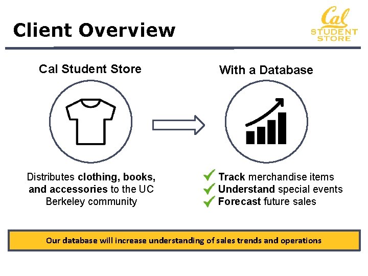
Client Overview Cal Student Store Distributes clothing, books, and accessories to the UC Berkeley community With a Database Track merchandise items Understand special events Forecast future sales Our database will increase understanding of sales trends and operations
Report Content 1 Client Summary 2 Database Design 3 SQL Queries 4 Normalization
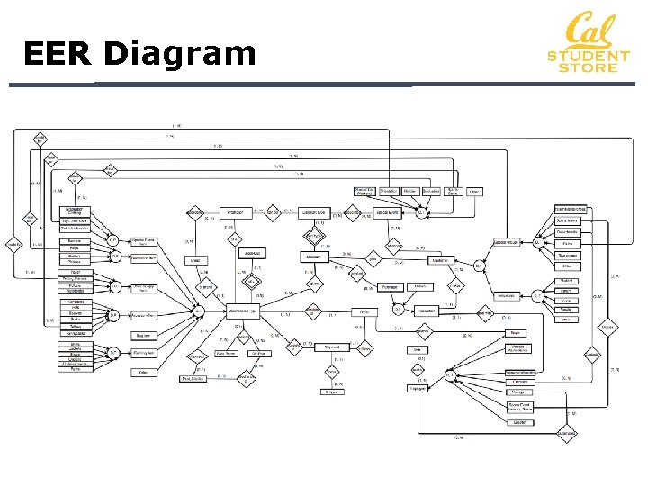
EER Diagram
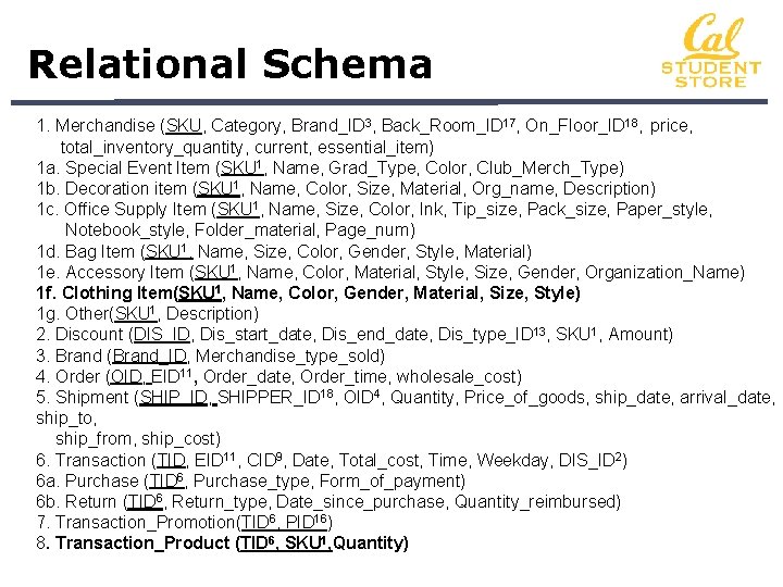
Relational Schema 1. Merchandise (SKU, Category, Brand_ID 3, Back_Room_ID 17, On_Floor_ID 18, price, total_inventory_quantity, current, essential_item) 1 a. Special Event Item (SKU 1, Name, Grad_Type, Color, Club_Merch_Type) 1 b. Decoration item (SKU 1, Name, Color, Size, Material, Org_name, Description) 1 c. Office Supply Item (SKU 1, Name, Size, Color, Ink, Tip_size, Pack_size, Paper_style, Notebook_style, Folder_material, Page_num) 1 d. Bag Item (SKU 1, Name, Size, Color, Gender, Style, Material) 1 e. Accessory Item (SKU 1, Name, Color, Material, Style, Size, Gender, Organization_Name) 1 f. Clothing Item(SKU 1, Name, Color, Gender, Material, Size, Style) 1 g. Other(SKU 1, Description) 2. Discount (DIS_ID, Dis_start_date, Dis_end_date, Dis_type_ID 13, SKU 1, Amount) 3. Brand (Brand_ID, Merchandise_type_sold) 4. Order (OID, EID 11, Order_date, Order_time, wholesale_cost) 5. Shipment (SHIP_ID, SHIPPER_ID 18, OID 4, Quantity, Price_of_goods, ship_date, arrival_date, ship_to, ship_from, ship_cost) 6. Transaction (TID, EID 11, CID 9, Date, Total_cost, Time, Weekday, DIS_ID 2) 6 a. Purchase (TID 6, Purchase_type, Form_of_payment) 6 b. Return (TID 6, Return_type, Date_since_purchase, Quantity_reimbursed) 7. Transaction_Promotion(TID 6, PID 16) 8. Transaction_Product (TID 6, SKU 1, Quantity)
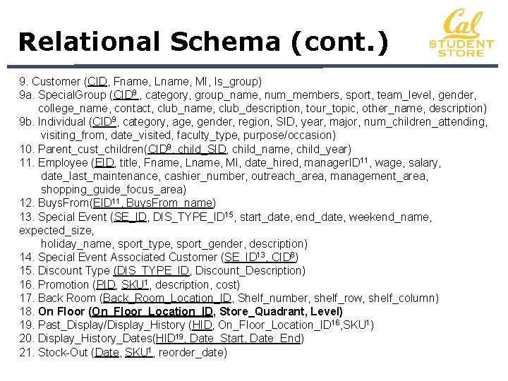
Relational Schema (cont. ) 9. Customer (CID, Fname, Lname, MI, Is_group) 9 a. Special. Group (CID 9 , category, group_name, num_members, sport, team_level, gender, college_name, contact, club_name, club_description, tour_topic, other_name, description) 9 b. Individual (CID 9, category, age, gender, region, SID, year, major, num_children_attending, visiting_from, date_visited, faculty_type, purpose/occasion) 10. Parent_cust_children(CID 9, child_SID, child_name, child_year) 11. Employee (EID, title, Fname, Lname, MI, date_hired, manager. ID 11, wage, salary, date_last_maintenance, cashier_number, outreach_area, management_area, shopping_guide_focus_area) 12. Buys. From(EID 11, Buys. From_name) 13. Special Event (SE_ID, DIS_TYPE_ID 15, start_date, end_date, weekend_name, expected_size, holiday_name, sport_type, sport_gender, description) 14. Special Event Associated Customer (SE_ID 13, CID 8) 15. Discount Type (DIS_TYPE_ID, Discount_Description) 16. Promotion (PID, SKU 1, description, cost) 17. Back Room (Back_Room_Location_ID, Shelf_number, shelf_row, shelf_column) 18. On Floor (On_Floor_Location_ID, Store_Quadrant, Level) 19. Past_Display/Display_History (HID, On_Floor_Location_ID 16, SKU 1) 20. Display_History_Dates(HID 19, Date_Start, Date_End) 21. Stock-Out (Date, SKU 1, reorder_date)
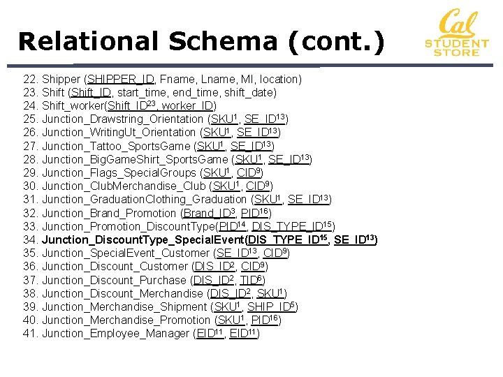
Relational Schema (cont. ) 22. Shipper (SHIPPER_ID, Fname, Lname, MI, location) 23. Shift (Shift_ID, start_time, end_time, shift_date) 24. Shift_worker(Shift_ID 23, worker_ID) 25. Junction_Drawstring_Orientation (SKU 1, SE_ID 13) 26. Junction_Writing. Ut_Orientation (SKU 1, SE_ID 13) 27. Junction_Tattoo_Sports. Game (SKU 1, SE_ID 13) 28. Junction_Big. Game. Shirt_Sports. Game (SKU 1, SE_ID 13) 29. Junction_Flags_Special. Groups (SKU 1, CID 9) 30. Junction_Club. Merchandise_Club (SKU 1, CID 9) 31. Junction_Graduation. Clothing_Graduation (SKU 1, SE_ID 13) 32. Junction_Brand_Promotion (Brand_ID 3, PID 16) 33. Junction_Promotion_Discount. Type(PID 14, DIS_TYPE_ID 15) 34. Junction_Discount. Type_Special. Event(DIS_TYPE_ID 15, SE_ID 13) 35. Junction_Special. Event_Customer (SE_ID 13, CID 9) 36. Junction_Discount_Customer (DIS_ID 2, CID 9) 37. Junction_Discount_Purchase (DIS_ID 2, TID 6) 38. Junction_Discount_Merchandise (DIS_ID 2, SKU 1) 39. Junction_Merchandise_Shipment (SKU 1, SHIP_ID 5) 40. Junction_Merchandise_Promotion (SKU 1, PID 16) 41. Junction_Employee_Manager (EID 11, EID 11)

Access Relationship View
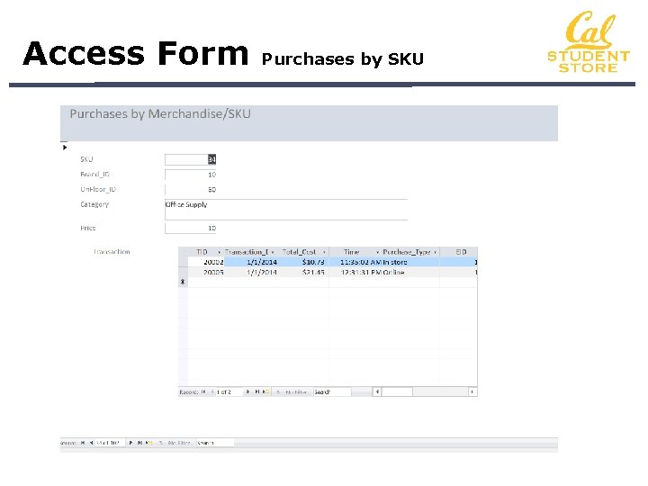
Access Form Purchases by SKU
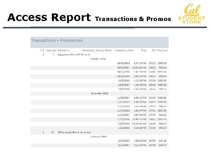
Access Report Transactions & Promos
Report Content 1 Client Summary 2 Database Design 3 SQL Queries 4 Normalization
Query #1 Worker Prediction Purpose: Run simulations to determine the optimal amount of workers Business Justification: Cal Student Store could save money by finding out when multiple workers are needed for peak times and only having extra workers for those hours Mathematical Model: Use Sigma and Simio with varying arrival times to determine the maximum number of workers needed at peak times based on demand Predict optimal number of workers Overview | Math | SQL | Results
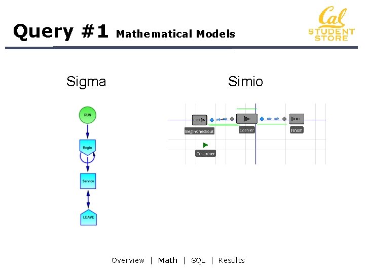
Query #1 Sigma Mathematical Models Simio Overview | Math | SQL | Results
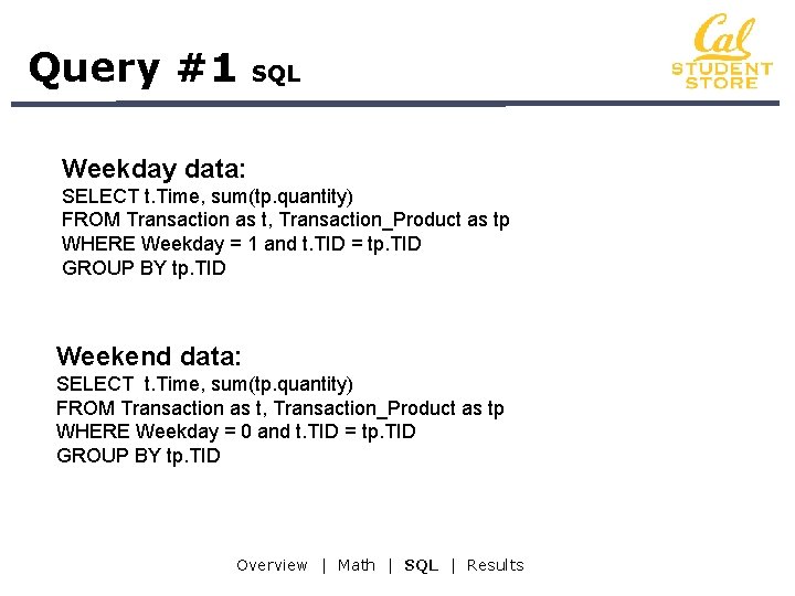
Query #1 SQL Weekday data: SELECT t. Time, sum(tp. quantity) FROM Transaction as t, Transaction_Product as tp WHERE Weekday = 1 and t. TID = tp. TID GROUP BY tp. TID Weekend data: SELECT t. Time, sum(tp. quantity) FROM Transaction as t, Transaction_Product as tp WHERE Weekday = 0 and t. TID = tp. TID GROUP BY tp. TID Overview | Math | SQL | Results
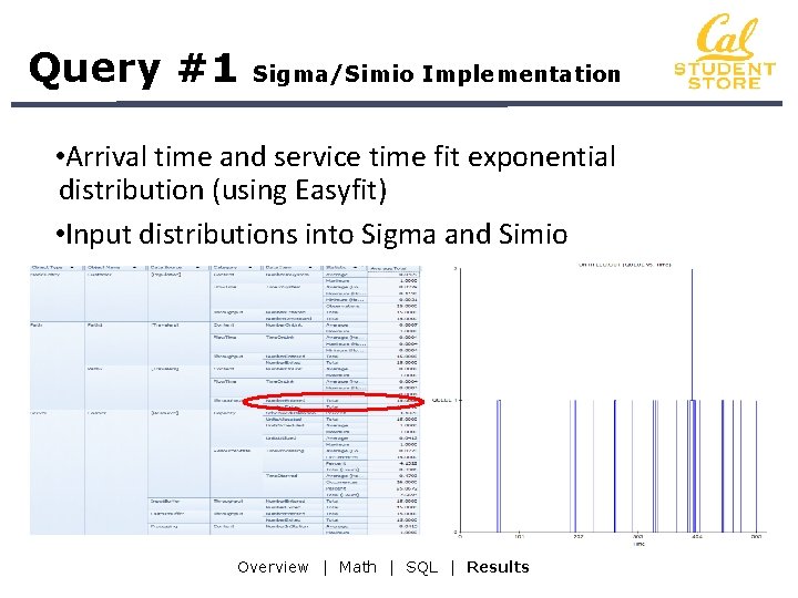
Query #1 Sigma/Simio Implementation • Arrival time and service time fit exponential distribution (using Easyfit) • Input distributions into Sigma and Simio Overview | Math | SQL | Results
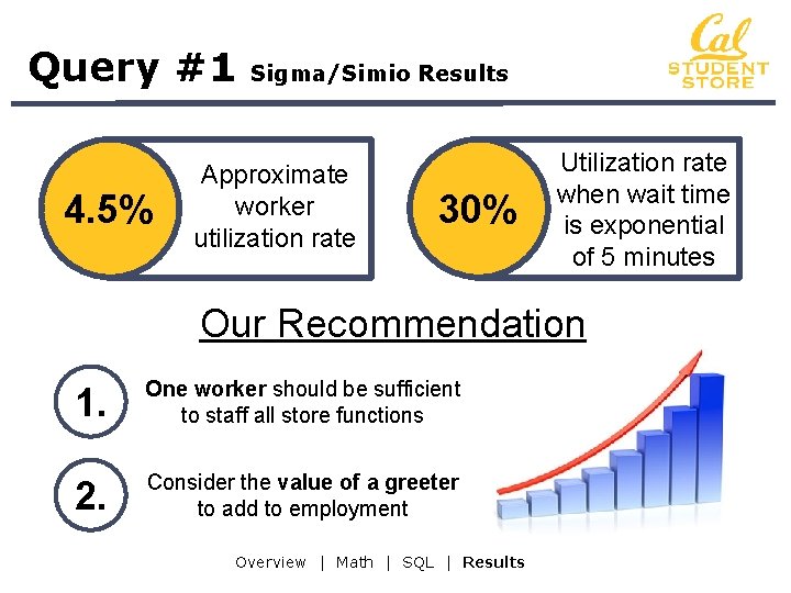
Query #1 4. 5% Sigma/Simio Results Approximate worker utilization rate 30% Utilization rate when wait time is exponential of 5 minutes Our Recommendation 1. One worker should be sufficient to staff all store functions 2. Consider the value of a greeter to add to employment Overview | Math | SQL | Results
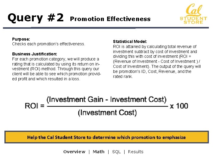
Query #2 Promotion Effectiveness Purpose: Checks each promotion’s effectiveness. Business Justification: For each promotion category, we will produce a rating that is calculated by using its return on investment (ROI) method. Through this query our client will be able to see which promotion provided profit and which resulted in a loss. Statistical Model: ROI is attained by calculating total revenue of investment subtract by cost of investment and dividing this with cost of investment (ROI = (Revenue of Investment - Cost of Investment ) / Cost of Investment). The output of the query will be promotion’s ID, Cost, Revenue, and the rated rank. Help the Cal Student Store to determine which promotion to emphasize Overview | Math | SQL | Results
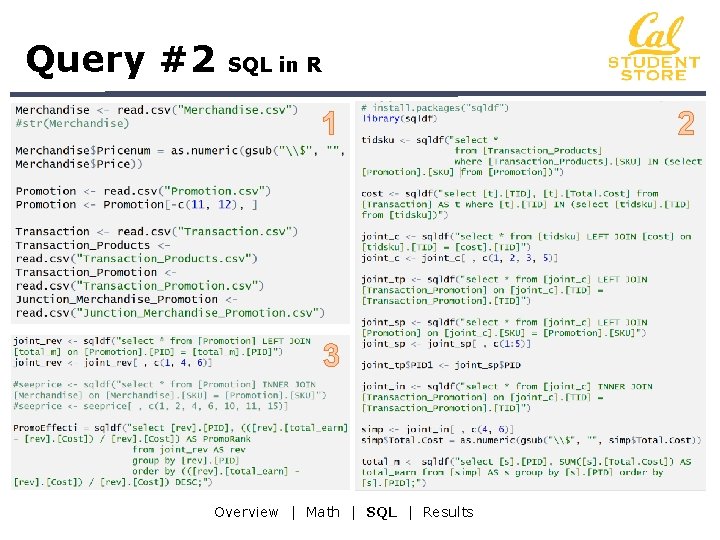
Query #2 SQL in R 11 2 3 Overview | Math | SQL | Results 2
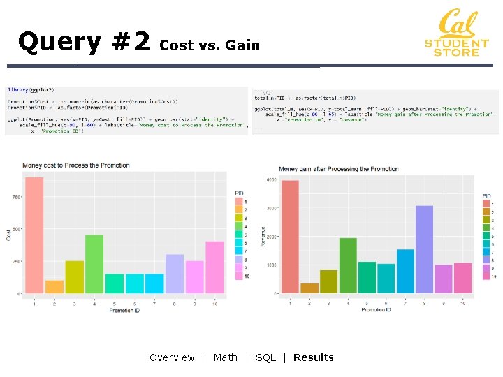
Query #2 Cost vs. Gain Overview | Math | SQL | Results
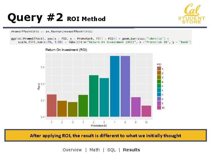
Query #2 ROI Method After applying ROI, the result is different to what we initially thought Overview | Math | SQL | Results
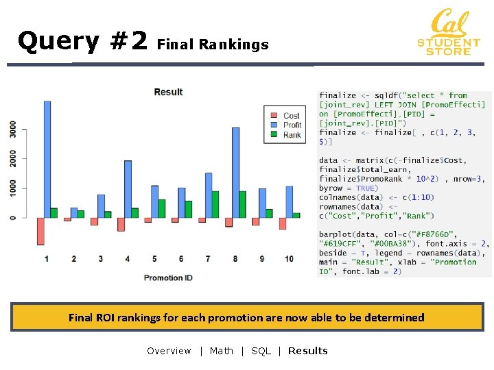
Query #2 Final Rankings Final ROI rankings for each promotion are now able to be determined Overview | Math | SQL | Results
Query #3 Product Location Purpose: Determine the most profitable way to place products in the on floor locations in the store. Business Justification: Running this query and performing the optimization allows the client to maximize profits by strategically placing products around the store, based on existing relationships between sales revenue and in-store location. Mathematical Model: Rank each in-store location’s optimal products by revenue generated, then solve a linear programming problem maximizing profit constrained by store space. Maximize revenue through optimal product in-store location Overview | Math | SQL | Results 24
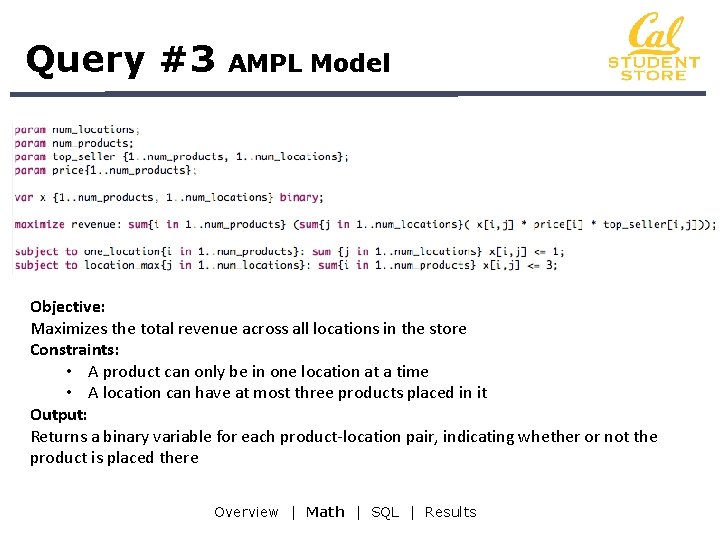
Query #3 AMPL Model Objective: Maximizes the total revenue across all locations in the store Constraints: • A product can only be in one location at a time • A location can have at most three products placed in it Output: Returns a binary variable for each product-location pair, indicating whether or not the product is placed there Overview | Math | SQL | Results
Query #3 SQL 1. ) Determine the Top 10 products for each on floor location: SELECT TOP 10 dh. ON_floor_location_ID AS Floor_Location, dh. SKU AS Product, AVG(tp. quantity * m. price) AS Revenue FROM Display_History AS dh, Display_History_Dates AS dhd, Merchandise AS m, On_Floor AS f, [Transaction] AS t, Transaction_Products AS tp WHERE dh. ON_floor_location_ID = 3 AND dh. HID = dhd. HID AND dh. SKU = tp. SKU AND m. SKU = tp. SKU AND tp. TID = t. TID AND t. date between dhd. Date_Start and dhd. Date_End GROUP BY dh. SKU, dh. ON_floor_location_ID; 2. ) Extract the prices of each product: SELECT SKU AS Product, price AS Product_Price FROM Merchandise; Overview | Math | SQL | Results
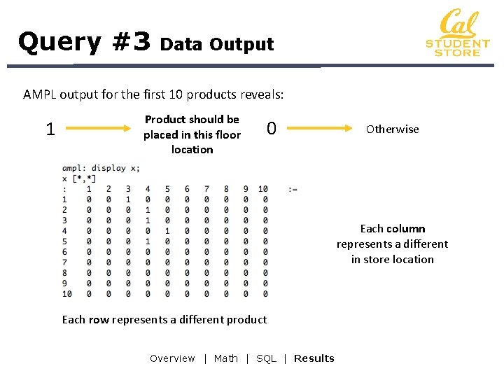
Query #3 Data Output AMPL output for the first 10 products reveals: 1 Product should be placed in this floor location 0 Otherwise Each column represents a different in store location Each row represents a different product Overview | Math | SQL | Results
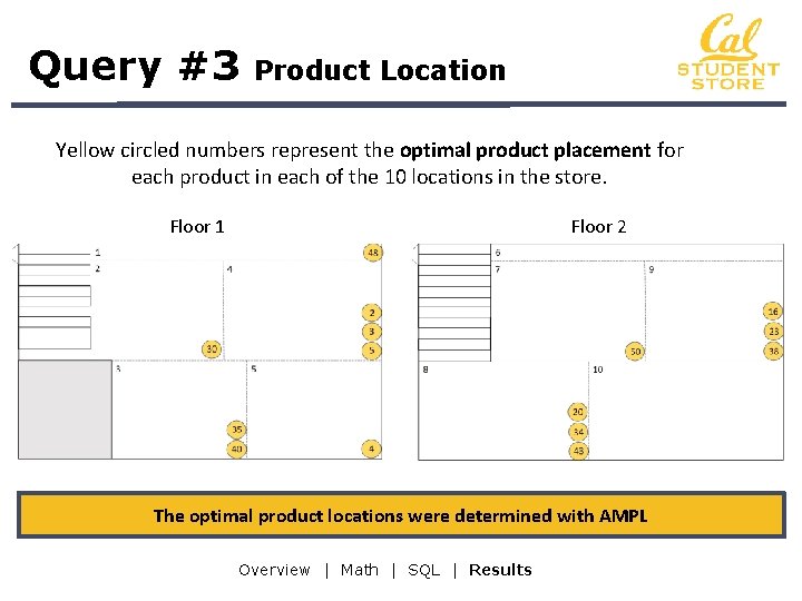
Query #3 Product Location Yellow circled numbers represent the optimal product placement for each product in each of the 10 locations in the store. Floor 2 Floor 1 The optimal product locations were determined with AMPL Overview | Math | SQL | Results
Query #4 Customer Behavior Prediction Purpose: Find out the category of products that are likely to be purchased by different customers, during both special and non-special event periods Business Justification: The Cal Student Store can recommend different products in their promotional emails, depending on different customer characteristics, to increase sales Mathematical Model: Used Machine Learning algorithms such as classification tree, linear modeling, and K-nearest-neighbor to predict customer behavior Implement more efficient marketing strategy based on customer behavior Overview | Math | SQL | Results
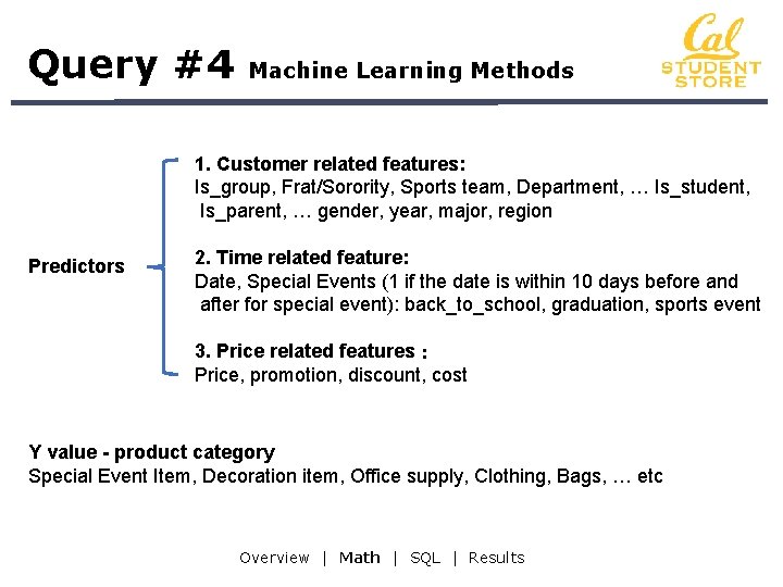
Query #4 Machine Learning Methods 1. Customer related features: Is_group, Frat/Sorority, Sports team, Department, … Is_student, Is_parent, … gender, year, major, region Predictors 2. Time related feature: Date, Special Events (1 if the date is within 10 days before and after for special event): back_to_school, graduation, sports event 3. Price related features: Price, promotion, discount, cost Y value - product category Special Event Item, Decoration item, Office supply, Clothing, Bags, … etc Overview | Math | SQL | Results
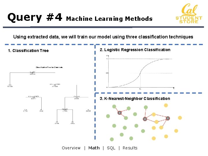
Query #4 Machine Learning Methods Using extracted data, we will train our model using three classification techniques 1. Classification Tree 2. Logistic Regression Classification 3. K-Nearest-Neighbor Classification Overview | Math | SQL | Results
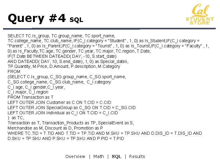
Query #4 SQL SELECT TC. Is_group, TC. group_name, TC. sport_name, TC. college_name, TC. club_name, IF(C_I. category = “Student” , 1, 0) as Is_Student, IF(C_I. category = “Parent” , 1, 0) as Is_Parent, IF(C_I. category = “Tourist” , 1, 0) as Is_Tourist, IF(C_I. category = “Faculty” , 1, 0) as Is_Faculty, TC. age, TC. gender, TC. year, TC. major, TC. region, T. Date, IF(T. Date BETWEEN DATEADD( DAY, -10, S. start_date) AND DATEADD( DAY, 10, S. end_date), 1, 0) as Special_dates, TP. Quantity, M. Price, D. Amount, P. description, M. Category FROM (SELECT C. Is_group, C_SG. group_name, C_SG. sport_name, C_SG. college_name, C_SG. club_name, C_I. category C_I. age, C_I. gender, C_I. year, C_I. major, C_I. region FROM Transaction as T LEFT OUTER JOIN Customer as C ON T. CID = C. CID LEFT OUTER JOIN Special. Group as C_SG ON T. CID = C_SG. CID LEFT OUTER JOIN Individual as C_I ON T. CID = C_I. CID ) as TC, Transaction as T, Transaction_Products as TP, Special. Event as S, Merchandise as M, Discount as D, Promotion as P WHERE TC. TID = T. TID AND T. TID = TP. TID AND M. SKU = TP. SKU AND D. DIS_ID = T. DIS_ID AND D. SKU = TP. SKU AND P. PID = T. PID Overview | Math | SQL | Results
Query #4 SQL Output Overview | Math | SQL | Results
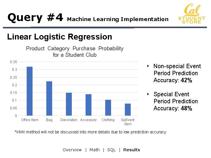
Query #4 Machine Learning Implementation Linear Logistic Regression Product Category Purchase Probability for a Student Club 0. 35 • Non-special Event Period Prediction Accuracy: 42% 0. 3 0. 25 0. 2 0. 15 • Special Event Period Prediction Accuracy: 48% 0. 1 0. 05 0 Office Item Bag Decoration Accessory Clothing Sp. Event Item *KNN method will not be discussed into more details due to low prediction accuracy Overview | Math | SQL | Results
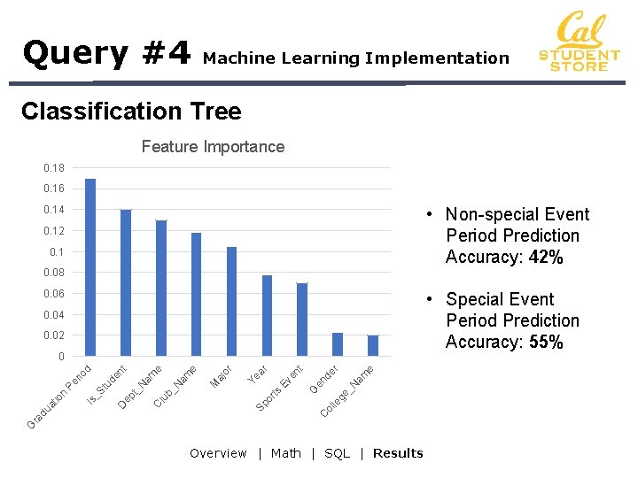
Query #4 Machine Learning Implementation Classification Tree Feature Importance 0. 18 0. 16 • Non-special Event Period Prediction Accuracy: 42% 0. 14 0. 12 0. 1 0. 08 0. 06 • Special Event Period Prediction Accuracy: 55% 0. 04 0. 02 e r _N am de en ol le ge G C Sp or ts Ev en t ar Ye M aj or e N am e b_ lu C D ep t_ N am nt de tu Is _S G ra d ua tio n Pe rio d 0 Overview | Math | SQL | Results
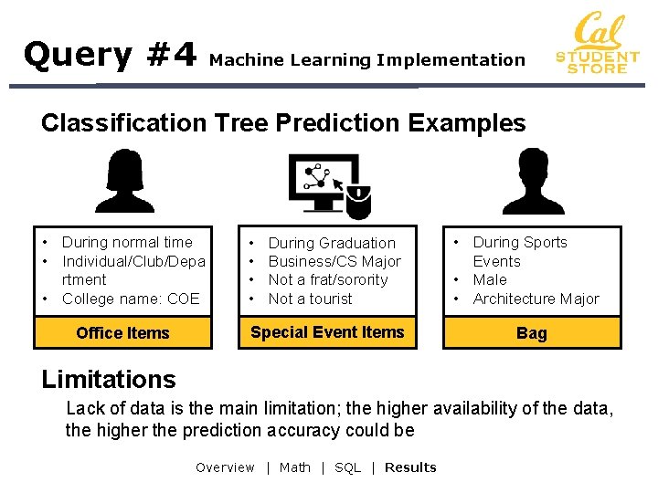
Query #4 Machine Learning Implementation Classification Tree Prediction Examples • During normal time • Individual/Club/Depa rtment • College name: COE Office Items • • During Graduation Business/CS Major Not a frat/sorority Not a tourist Special Event Items • During Sports Events • Male • Architecture Major Bag Limitations Lack of data is the main limitation; the higher availability of the data, the higher the prediction accuracy could be Overview | Math | SQL | Results
Query #5 Inventory Management Purpose: Conduct inventory analysis on time-sensitive products to determine the proper order/re-stock/stock-off time Business Justification: Allows Cal Student Store to predict the demand for time-sensitive products so that they can manage the inventory accordingly, given the spatial limit of the Cal Student Store’s storage facilities and set shipping times Statistical Model: Fit time series model on the existing data of demand for time-sensitive products to predict future trends, taking into consideration of possible seasonal fluctuation and effects from special events Help the Cal Student Store strategically place orders and clear inventory Overview | Math | SQL | Results
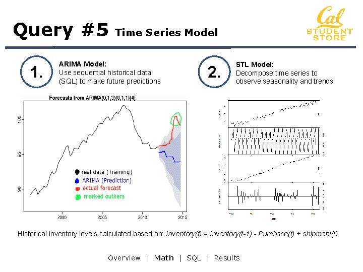
Query #5 1. Time Series Model ARIMA Model: Use sequential historical data (SQL) to make future predictions 2. STL Model: Decompose time series to observe seasonality and trends Historical inventory levels calculated based on: Inventory(t) = Inventory(t-1) - Purchase(t) + shipment(t) Overview | Math | SQL | Results
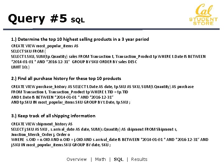
Query #5 SQL 1. ) Determine the top 10 highest selling products in a 3 year period CREATE VIEW most_popular_items AS SELECT SKU FROM ( SELECT t. SKU, SUM(tp. Quantity) sales FROM Transaction t, Transaction_Product tp WHERE t. Date IS BETWEEN “ 2014 -01 -01 “ AND “ 2016 -12 -31” GROUP BY SKU ORDER BY sales DESC LIMIT 10; ) 2. ) Find all purchase history for these top 10 products CREATE VIEW purchase_history AS SELECT t. Date AS date, tp. SKU AS SKU, SUM(t. Quantity) AS purchase FROM Transaction t, Transaction_Product tp WHERE t. TID = tp. TID AND t. Date IS BETWEEN “ 2014 -01 -01 “ AND “ 2016 -12 -31” AND tp. SKU IN most_popular_items. SKU GROUP BY t. Date, tp. SKU ; 3. ) Keep track of all shipping information CREATE VIEW shipment_history AS SELECT j. SKU AS SKU , s. arrival_date AS date, SUM(s. Quantity) AS shipment FROM Shipment s, Junction_Merch_Order j, Order o WHERE s. OID = o. OID AND o. OID = j. OID AND s. arrival_date IS BETWEEN “ 2014 -01 -01 “ AND “ 2016 -12 -31” AND j. SKU IN most_popular_items. SKU GROUP BY date, SKU ; Overview | Math | SQL | Results
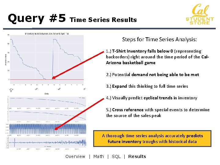
Query #5 Time Series Results Steps for Time Series Analysis: 1. ) T-Shirt Inventory falls below 0 (representing backorders) right around the time period of the Cal. Arizona basketball game 2. ) Potential demand not being able to be met 3. ) Expand this thinking to full time series 4. ) Visually predict cyclical trends in inventory 5. ) Cross reference with special events to determine the source of the sales peak A thorough time series analysis accurately predicts future inventory troughs with historical data Overview | Math | SQL | Results
Report Content 1 Client Summary 2 Database Design 3 SQL Queries 4 Normalization
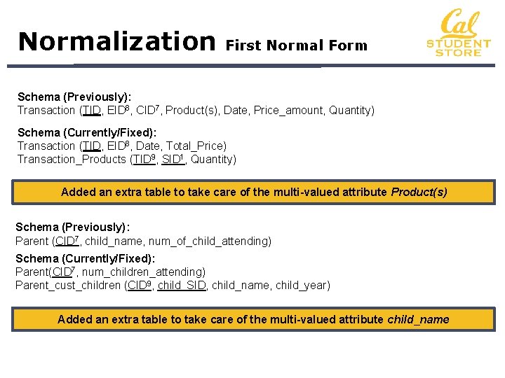
Normalization First Normal Form Schema (Previously): Transaction (TID, EID 8, CID 7, Product(s), Date, Price_amount, Quantity) Schema (Currently/Fixed): Transaction (TID, EID 8, Date, Total_Price) Transaction_Products (TID 9, SID 1, Quantity) Added an extra table to take care of the multi-valued attribute Product(s) Schema (Previously): Parent (CID 7, child_name, num_of_child_attending) Schema (Currently/Fixed): Parent(CID 7, num_children_attending) Parent_cust_children (CID 9, child_SID, child_name, child_year) Added an extra table to take care of the multi-valued attribute child_name
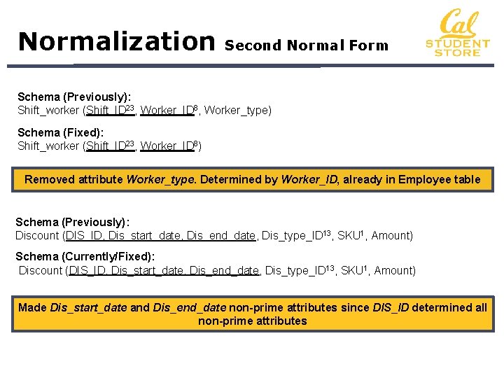
Normalization Second Normal Form Schema (Previously): Shift_worker (Shift_ID 23, Worker_ID 8, Worker_type) Schema (Fixed): Shift_worker (Shift_ID 23, Worker_ID 8) Removed attribute Worker_type. Determined by Worker_ID, already in Employee table Schema (Previously): Discount (DIS_ID, Dis_start_date, Dis_end_date, Dis_type_ID 13, SKU 1, Amount) Schema (Currently/Fixed): Discount (DIS_ID, Dis_start_date, Dis_end_date, Dis_type_ID 13, SKU 1, Amount) Made Dis_start_date and Dis_end_date non-prime attributes since DIS_ID determined all non-prime attributes
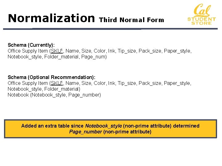
Normalization Third Normal Form Schema (Currently): Office Supply Item (SKU 1, Name, Size, Color, Ink, Tip_size, Pack_size, Paper_style, Notebook_style, Folder_material, Page_num) Schema (Optional Recommendation): Office Supply Item (SKU 1, Name, Size, Color, Ink, Tip_size, Pack_size, Paper_style, Notebook_style, Folder_material) Notebook (Notebook_style, Page_number) Added an extra table since Notebook_style (non-prime attribute) determined Page_number (non-prime attribute)
THANK YOU!
- Slides: 45