Data Warehousing Need for Speed Parallelism Data Warehousing

Data Warehousing Need for Speed: Parallelism Data Warehousing 1

Background 2 Data Warehousing

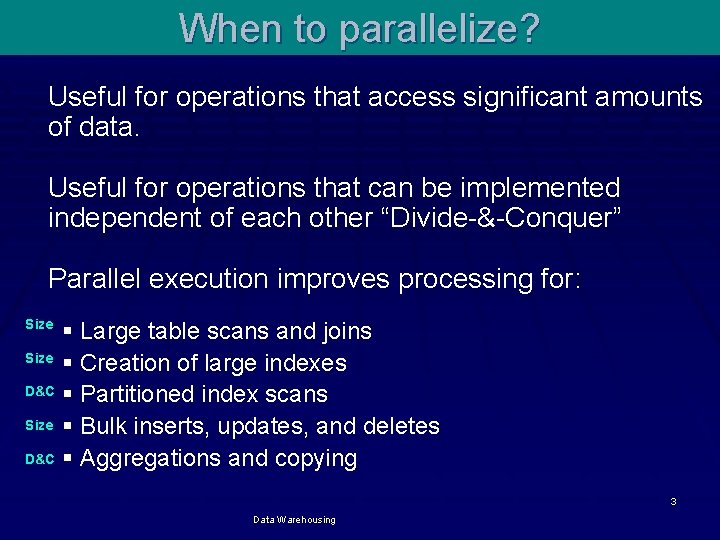
When to parallelize? Useful for operations that access significant amounts of data. Useful for operations that can be implemented independent of each other “Divide-&-Conquer” Parallel execution improves processing for: Size § Large table scans and joins Size § Creation of large indexes D&C § Partitioned index scans Size § Bulk inserts, updates, and deletes D&C § Aggregations and copying 3 Data Warehousing

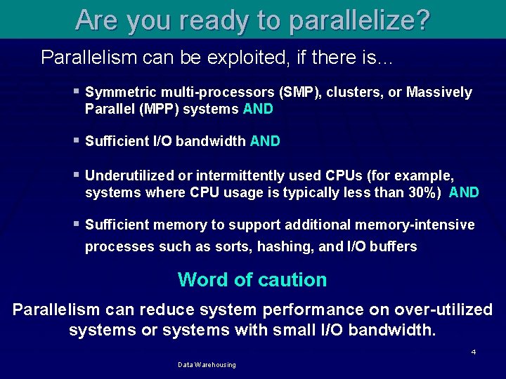
Are you ready to parallelize? Parallelism can be exploited, if there is… § Symmetric multi-processors (SMP), clusters, or Massively Parallel (MPP) systems AND § Sufficient I/O bandwidth AND § Underutilized or intermittently used CPUs (for example, systems where CPU usage is typically less than 30%) AND § Sufficient memory to support additional memory-intensive processes such as sorts, hashing, and I/O buffers Word of caution Parallelism can reduce system performance on over-utilized systems or systems with small I/O bandwidth. 4 Data Warehousing

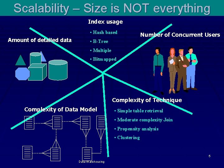
Scalability – Size is NOT everything Index usage • Hash based Amount of detailed data Number of Concurrent Users • B-Tree • Multiple • Bitmapped Complexity of Technique Complexity of Data Model • Simple table retrieval • Moderate complexity Join • Propensity analysis • Clustering Data Warehousing 5

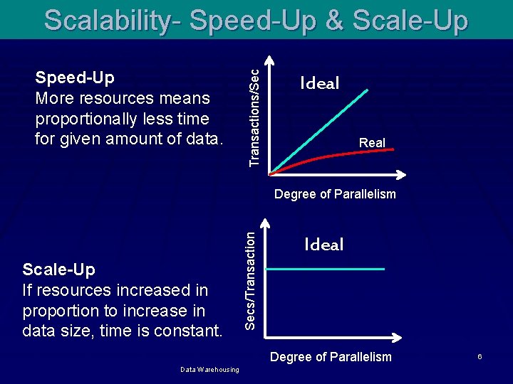
Speed-Up More resources means proportionally less time for given amount of data. Transactions/Sec Scalability- Speed-Up & Scale-Up Ideal Real Scale-Up If resources increased in proportion to increase in data size, time is constant. Secs/Transaction Degree of Parallelism Ideal Degree of Parallelism Data Warehousing 6

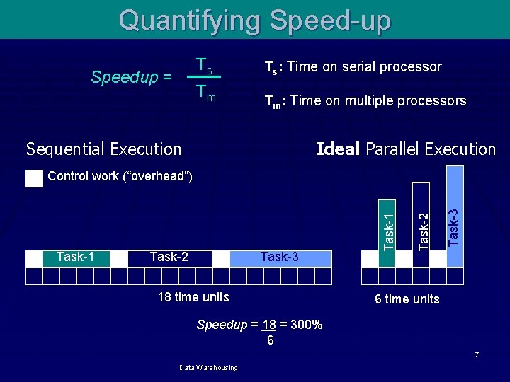
Quantifying Speed-up Ts Speedup = Tm Ts: Time on serial processor Tm: Time on multiple processors Sequential Execution Ideal Parallel Execution Task-2 Task-3 18 time units Task-3 Task-2 Task-1 Control work (“overhead”) 6 time units Speedup = 18 = 300% 6 7 Data Warehousing

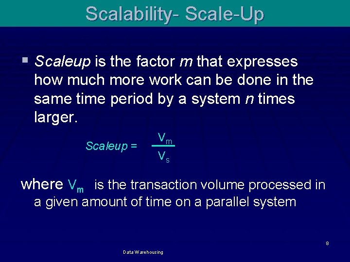
Scalability- Scale-Up § Scaleup is the factor m that expresses how much more work can be done in the same time period by a system n times larger. Scaleup = Vm Vs where Vm is the transaction volume processed in a given amount of time on a parallel system 8 Data Warehousing

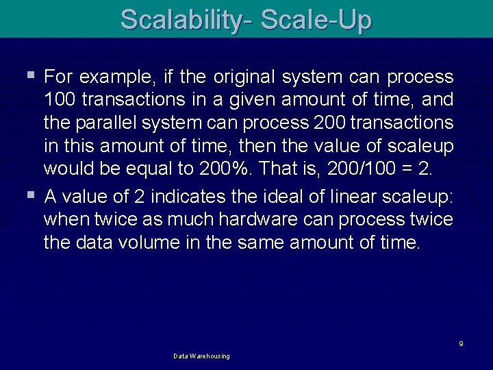
Scalability- Scale-Up § For example, if the original system can process 100 transactions in a given amount of time, and the parallel system can process 200 transactions in this amount of time, then the value of scaleup would be equal to 200%. That is, 200/100 = 2. § A value of 2 indicates the ideal of linear scaleup: when twice as much hardware can process twice the data volume in the same amount of time. 9 Data Warehousing

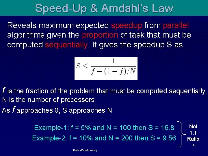
Speed-Up & Amdahl’s Law Reveals maximum expected speedup from parallel algorithms given the proportion of task that must be computed sequentially. It gives the speedup S as f is the fraction of the problem that must be computed sequentially N is the number of processors As f approaches 0, S approaches N Example-1: f = 5% and N = 100 then S = 16. 8 Example-2: f = 10% and N = 200 then S = 9. 56 Not 1: 1 Ratio 10 Data Warehousing

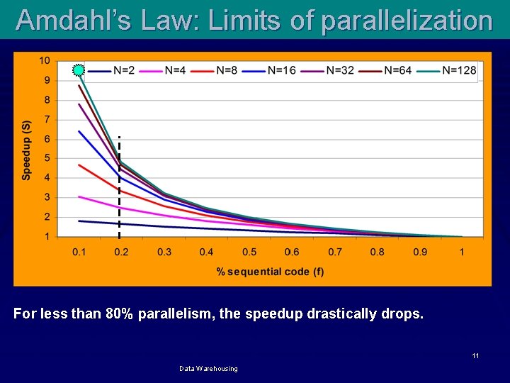
Amdahl’s Law: Limits of parallelization For less than 80% parallelism, the speedup drastically drops. 11 Data Warehousing

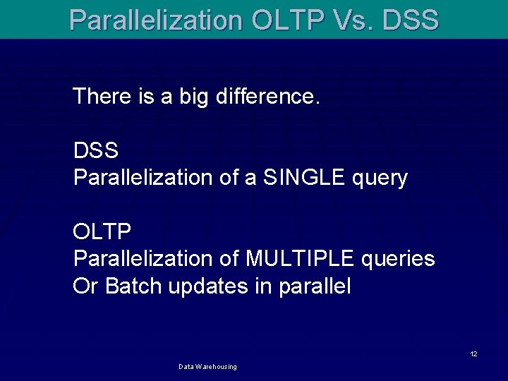
Parallelization OLTP Vs. DSS There is a big difference. DSS Parallelization of a SINGLE query OLTP Parallelization of MULTIPLE queries Or Batch updates in parallel 12 Data Warehousing

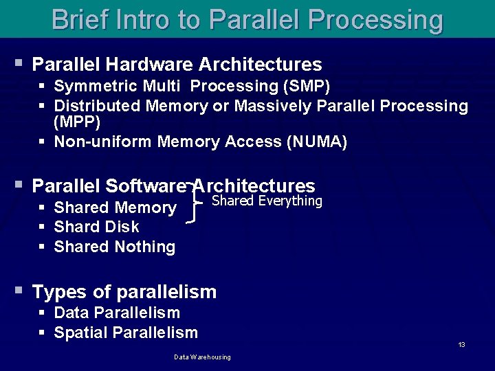
Brief Intro to Parallel Processing § Parallel Hardware Architectures § Symmetric Multi Processing (SMP) § Distributed Memory or Massively Parallel Processing (MPP) § Non-uniform Memory Access (NUMA) § Parallel Software Architectures § § § Shared Memory Shard Disk Shared Nothing Shared Everything § Types of parallelism § § Data Parallelism Spatial Parallelism Data Warehousing 13

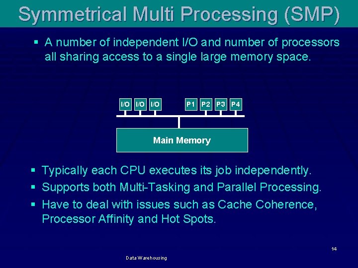
Symmetrical Multi Processing (SMP) § A number of independent I/O and number of processors all sharing access to a single large memory space. I/O I/O P 1 P 2 P 3 P 4 Main Memory § Typically each CPU executes its job independently. § Supports both Multi-Tasking and Parallel Processing. § Have to deal with issues such as Cache Coherence, Processor Affinity and Hot Spots. 14 Data Warehousing

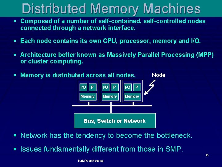
Distributed Memory Machines § Composed of a number of self-contained, self-controlled nodes connected through a network interface. § Each node contains its own CPU, processor, memory and I/O. § Architecture better known as Massively Parallel Processing (MPP) or cluster computing. § Memory is distributed across all nodes. I/O P Memory I/O Node P Memory Bus, Switch or Network § Network has the tendency to become the bottleneck. § Issues fundamentally different from those in SMP. Data Warehousing 15

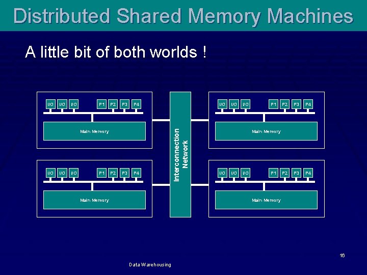
Distributed Shared Memory Machines A little bit of both worlds ! I/O P 1 P 2 P 3 Main Memory I/O I/O P 1 P 2 P 3 I/O P 4 Main Memory Interconnection Network I/O I/O P 1 P 2 P 3 P 4 Main Memory I/O I/O P 1 Main Memory 16 Data Warehousing

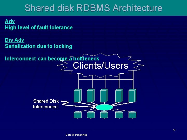
Shared disk RDBMS Architecture Adv High level of fault tolerance Dis Adv Serialization due to locking Interconnect can become a bottleneck Clients/Users Shared Disk Interconnect 17 Data Warehousing

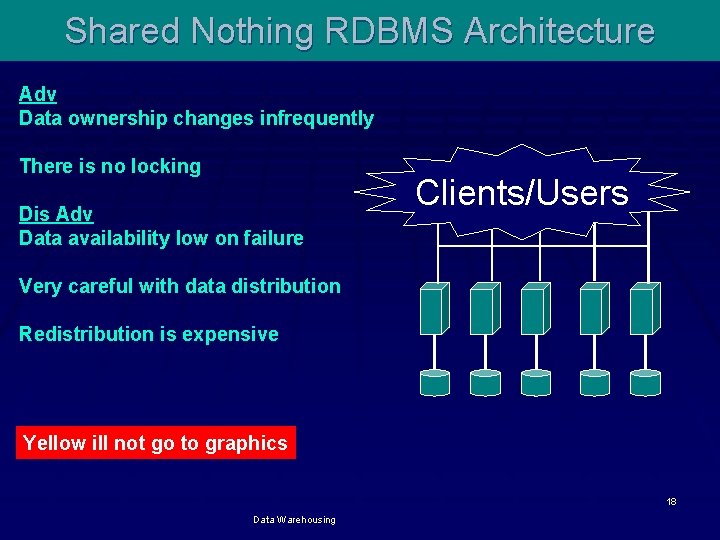
Shared Nothing RDBMS Architecture Adv Data ownership changes infrequently There is no locking Dis Adv Data availability low on failure Clients/Users Very careful with data distribution Redistribution is expensive Yellow ill not go to graphics 18 Data Warehousing

Shared disk Vs. Shared Nothing RDBMS § Important note: Do not confuse RDBMS architecture with hardware architecture. § Shared nothing databases can run on shared everything (SMP or NUMA) hardware. § Shared disk databases can run on shared nothing (MPP) hardware. This slide will not go to graphics 19 Data Warehousing

Parallelism Methodologies Data Warehousing 20

Motivation § No need of parallelism if perfect computer § with single infinitely fast processor § with an infinite memory with infinite bandwidth § and its infinitely cheap too (free!) § Technology is not delivering (going to Moon analogy) § The Challenge is to build § infinitely fast processor out of infinitely many processors of finite speed No text goes to graphics § Infinitely large memory with infinite memory bandwidth from infinite many finite storage units of finite speed 21 Data Warehousing

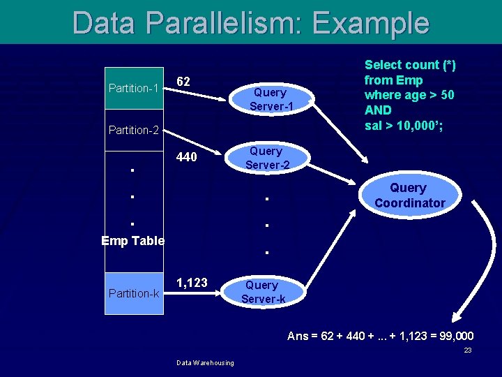
Data Parallelism: Concept § Parallel execution of a single data manipulation task across multiple partitions of data. § Partitions static or dynamic § Tasks executed almost-independently across partitions. § “Query coordinator” must coordinate between the independently executing processes. 22 Data Warehousing

Data Parallelism: Example Partition 1 Partition-1 62 Query Server-1 Partition-2 . . . 440 Partition-k Query Server-2 . . . Emp Table 1, 123 Select count (*) from Emp where age > 50 AND sal > 10, 000’; Query Coordinator Query Server-k Ans = 62 + 440 +. . . + 1, 123 = 99, 000 23 Data Warehousing

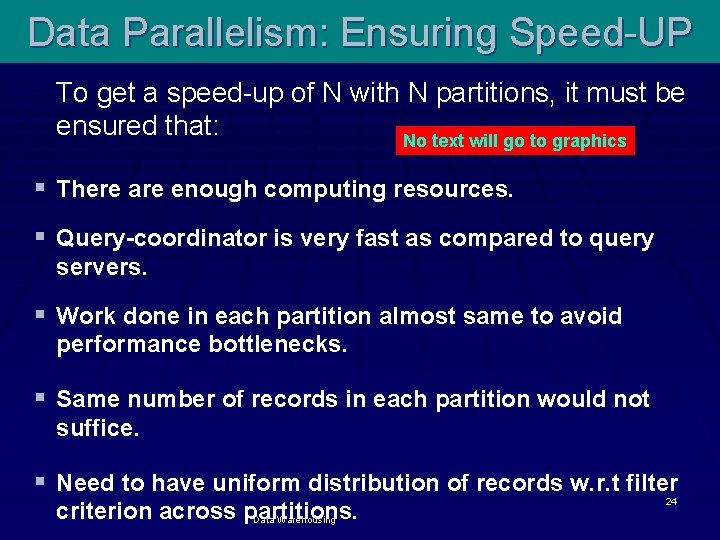
Data Parallelism: Ensuring Speed-UP To get a speed-up of N with N partitions, it must be ensured that: No text will go to graphics § There are enough computing resources. § Query-coordinator is very fast as compared to query servers. § Work done in each partition almost same to avoid performance bottlenecks. § Same number of records in each partition would not suffice. § Need to have uniform distribution of records w. r. t filter criterion across partitions. Data Warehousing 24

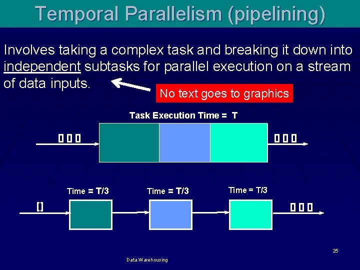
Temporal Parallelism (pipelining) Involves taking a complex task and breaking it down into independent subtasks for parallel execution on a stream of data inputs. No text goes to graphics Task Execution Time = T [] [] [] Time = T/3 [] [] [] 25 Data Warehousing

Pipelining: Time Chart Time = T/3 Time = T/3 [] [] Time = T/3 [] Time = T/3 [] T=0 T=1 T=2 T=3 26 Data Warehousing

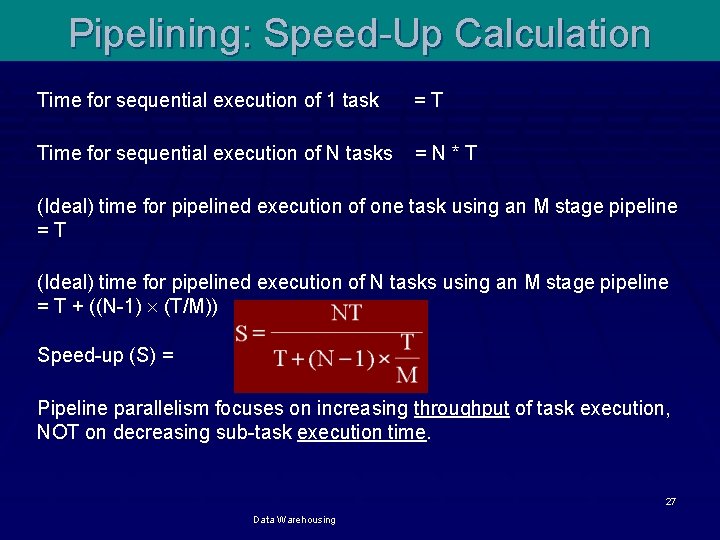
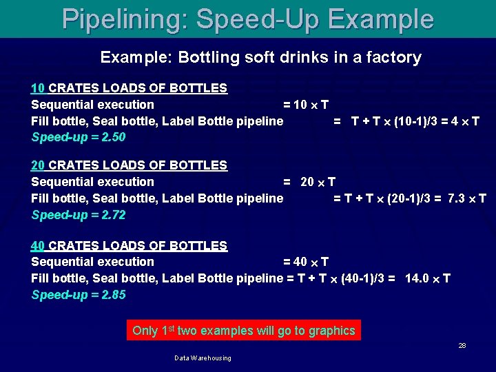
Pipelining: Speed-Up Calculation Time for sequential execution of 1 task =T Time for sequential execution of N tasks =N*T (Ideal) time for pipelined execution of one task using an M stage pipeline =T (Ideal) time for pipelined execution of N tasks using an M stage pipeline = T + ((N-1) (T/M)) Speed-up (S) = Pipeline parallelism focuses on increasing throughput of task execution, NOT on decreasing sub-task execution time. 27 Data Warehousing

Pipelining: Speed-Up Example: Bottling soft drinks in a factory 10 CRATES LOADS OF BOTTLES Sequential execution = 10 T Fill bottle, Seal bottle, Label Bottle pipeline = T + T (10 -1)/3 = 4 T Speed-up = 2. 50 20 CRATES LOADS OF BOTTLES Sequential execution = 20 T Fill bottle, Seal bottle, Label Bottle pipeline = T + T (20 -1)/3 = 7. 3 T Speed-up = 2. 72 40 CRATES LOADS OF BOTTLES Sequential execution = 40 T Fill bottle, Seal bottle, Label Bottle pipeline = T + T (40 -1)/3 = 14. 0 T Speed-up = 2. 85 Only 1 st two examples will go to graphics 28 Data Warehousing

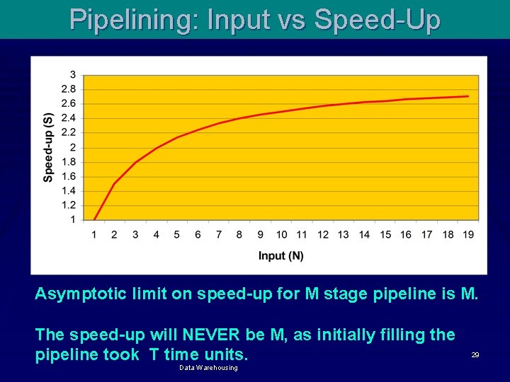
Pipelining: Input vs Speed-Up Asymptotic limit on speed-up for M stage pipeline is M. The speed-up will NEVER be M, as initially filling the pipeline took T time units. Data Warehousing 29

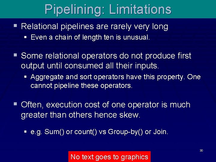
Pipelining: Limitations § Relational pipelines are rarely very long § Even a chain of length ten is unusual. § Some relational operators do not produce first output until consumed all their inputs. § Aggregate and sort operators have this property. One cannot pipeline these operators. § Often, execution cost of one operator is much greater than others hence skew. § e. g. Sum() or count() vs Group-by() or Join. 30 Data Warehousing No text goes to graphics

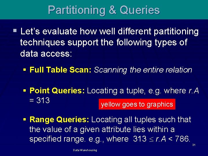
Partitioning & Queries § Let’s evaluate how well different partitioning techniques support the following types of data access: § Full Table Scan: Scanning the entire relation § Point Queries: Locating a tuple, e. g. where r. A = 313 yellow goes to graphics § Range Queries: Locating all tuples such that the value of a given attribute lies within a specified range. e. g. , where 313 r. A < 786. Data Warehousing 31

Partitioning & Queries Round Robin § Advantages § Best suited for sequential scan of entire relation on each query. yellow goes to graphics § All disks have almost an equal number of tuples; retrieval work is thus well balanced between disks. § Range queries are difficult to process § No clustering -- tuples are scattered across all disks 32 Data Warehousing

Partitioning & Queries Hash Partitioning § Good for sequential access § With uniform hashing and using partitioning attributes as a key, tuples will be equally distributed between disks. § Good for point queries on partitioning attribute § Can lookup single disk, leaving others available for answering other queries. yellow goes to graphics § Index on partitioning attribute can be local to disk, making lookup and update very efficient even joins. • Range queries are difficult to process No clustering -- tuples are scattered across all Data Warehousing disks 33

Partitioning & Queries Range Partitioning § Provides data clustering by partitioning attribute value. § Good for sequential access yellow goes to graphics § Good for point queries on partitioning attribute: only one disk needs to be accessed. § For range queries on partitioning attribute, one or a few disks may need to be accessed - Remaining disks are available for other queries. - Good if result tuples are from one to a few blocks. - If many blocks are to be fetched, they are still fetched from one to a few disks, then potential parallelism in disk access is wasted 34 Data Warehousing

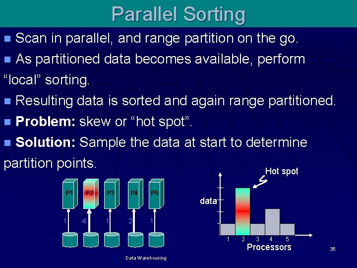
Parallel Sorting Scan in parallel, and range partition on the go. n As partitioned data becomes available, perform “local” sorting. n Resulting data is sorted and again range partitioned. n Problem: skew or “hot spot”. n Solution: Sample the data at start to determine partition points Hot spot n P 1 1 P 2 4 P 3 1 P 4 2 P 5 data 1 1 Data Warehousing 2 3 4 5 Processors 35

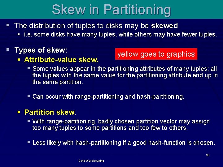
Skew in Partitioning § The distribution of tuples to disks may be skewed § i. e. some disks have many tuples, while others may have fewer tuples. § Types of skew: yellow goes to graphics § Attribute-value skew. § Some values appear in the partitioning attributes of many tuples; all the tuples with the same value for the partitioning attribute end up in the same partition. § Can occur with range-partitioning and hash-partitioning. § Partition skew. § With range-partitioning, badly chosen partition vector may assign too many tuples to some partitions and too few to others. § Less likely with hash-partitioning if a good hash-function is chosen. 36 Data Warehousing

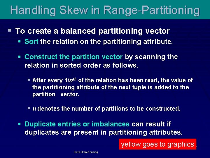
Handling Skew in Range-Partitioning § To create a balanced partitioning vector § Sort the relation on the partitioning attribute. § Construct the partition vector by scanning the relation in sorted order as follows. § After every 1/nth of the relation has been read, the value of the partitioning attribute of the next tuple is added to the partition vector. § n denotes the number of partitions to be constructed. § Duplicate entries or imbalances can result if duplicates are present in partitioning attributes. yellow goes to graphics 37 Data Warehousing

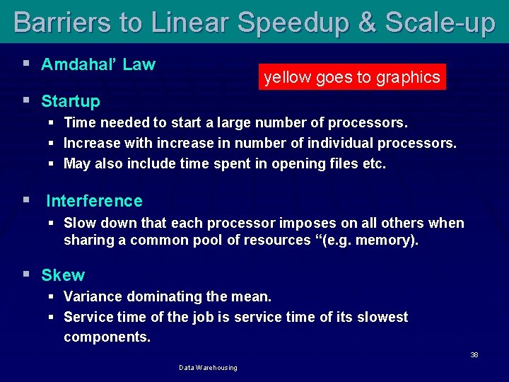
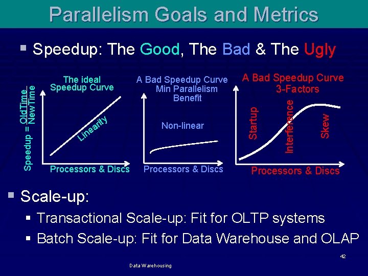
Barriers to Linear Speedup & Scale-up § Amdahal’ Law yellow goes to graphics § Startup § Time needed to start a large number of processors. § Increase with increase in number of individual processors. § May also include time spent in opening files etc. § Interference § Slow down that each processor imposes on all others when sharing a common pool of resources “(e. g. memory). § Skew § Variance dominating the mean. § Service time of the job is service time of its slowest components. 38 Data Warehousing

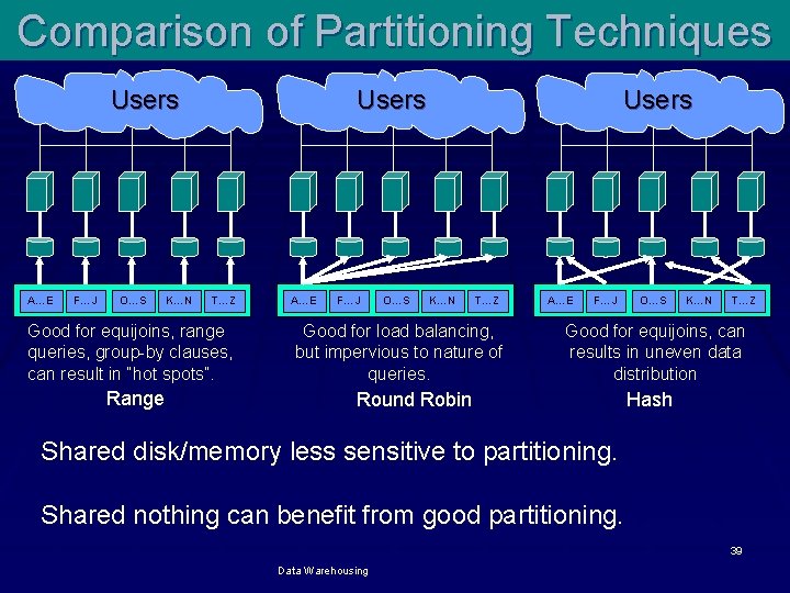
Comparison of Partitioning Techniques Users A…E F…J O…S K…N T…Z Good for equijoins, range queries, group-by clauses, can result in “hot spots”. Range A…E F…J O…S Users K…N T…Z Good for load balancing, but impervious to nature of queries. A…E F…J O…S K…N T…Z Good for equijoins, can results in uneven data distribution Round Robin Hash Shared disk/memory less sensitive to partitioning. Shared nothing can benefit from good partitioning. 39 Data Warehousing

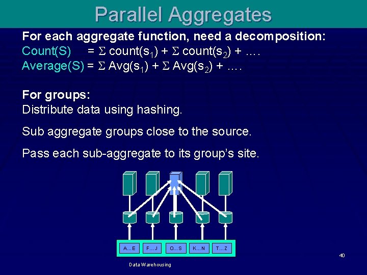
Parallel Aggregates For each aggregate function, need a decomposition: Count(S) = count(s 1) + count(s 2) + …. Average(S) = Avg(s 1) + Avg(s 2) + …. For groups: Distribute data using hashing. Sub aggregate groups close to the source. Pass each sub-aggregate to its group’s site. A…E F…J O…S K…N T…Z 40 Data Warehousing

When to use which partitioning Tech? § When to use Range Partitioning? § When to Use Hash Partitioning? § When to Use List Partitioning? § When to use Round-Robin Partitioning? 41 Data Warehousing

Parallelism Goals and Metrics y Non-linear Lin Processors & Discs A Bad Speedup Curve 3 -Factors Skew rit a e A Bad Speedup Curve Min Parallelism Benefit Interference The ideal Speedup Curve Startup Old. Time Speedup = New. Time § Speedup: The Good, The Bad & The Ugly Processors & Discs § Scale-up: § Transactional Scale-up: Fit for OLTP systems § Batch Scale-up: Fit for Data Warehouse and OLAP 42 Data Warehousing