Data Warehousing and Data Mining Chapter 3 Data

Data Warehousing and Data Mining — Chapter 3 — — Data Preprocessing — 2013/2014 Fall 1

Chapter 3: Data Preprocessing n Why preprocess the data? n Data cleaning n Data integration and transformation n Data reduction n Discretization and concept hierarchy generation n Time-dependent data n Summary 2

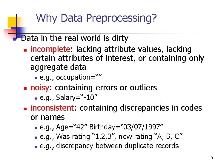
Why Data Preprocessing? n Data in the real world is dirty n incomplete: lacking attribute values, lacking certain attributes of interest, or containing only aggregate data n n noisy: containing errors or outliers n n e. g. , occupation=“” e. g. , Salary=“-10” inconsistent: containing discrepancies in codes or names n n n e. g. , Age=“ 42” Birthday=“ 03/07/1997” e. g. , Was rating “ 1, 2, 3”, now rating “A, B, C” e. g. , discrepancy between duplicate records 3

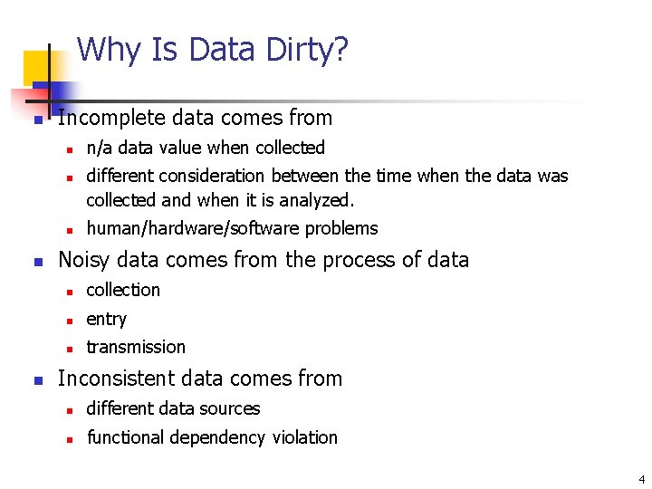
Why Is Data Dirty? n Incomplete data comes from n n n/a data value when collected different consideration between the time when the data was collected and when it is analyzed. human/hardware/software problems Noisy data comes from the process of data n collection n entry n transmission Inconsistent data comes from n different data sources n functional dependency violation 4

Why Is Data Preprocessing Important? n No quality data, no quality mining results! n Quality decisions must be based on quality data n n n e. g. , duplicate or missing data may cause incorrect or even misleading statistics. Data warehouse needs consistent integration of quality data Data extraction, cleaning, and transformation comprises the majority of the work of building a data warehouse 5

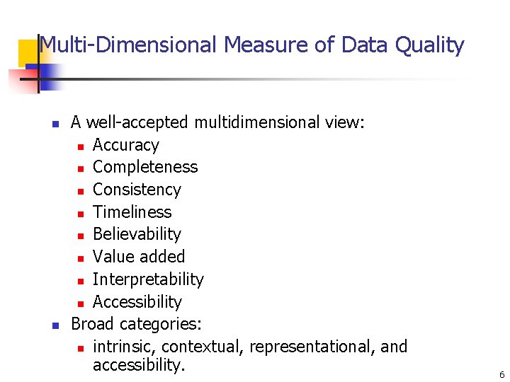
Multi-Dimensional Measure of Data Quality n n A well-accepted multidimensional view: n Accuracy n Completeness n Consistency n Timeliness n Believability n Value added n Interpretability n Accessibility Broad categories: n intrinsic, contextual, representational, and accessibility. 6

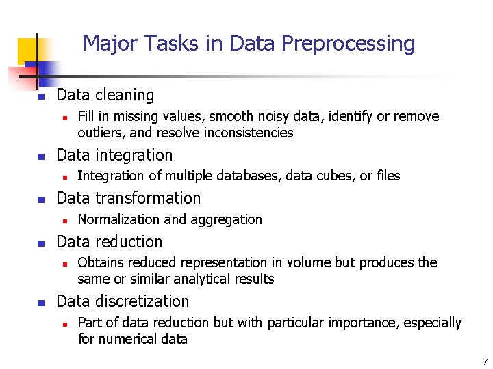
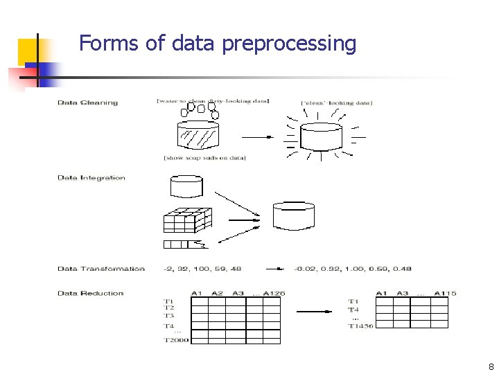
Major Tasks in Data Preprocessing n Data cleaning n n Data integration n n Normalization and aggregation Data reduction n n Integration of multiple databases, data cubes, or files Data transformation n n Fill in missing values, smooth noisy data, identify or remove outliers, and resolve inconsistencies Obtains reduced representation in volume but produces the same or similar analytical results Data discretization n Part of data reduction but with particular importance, especially for numerical data 7

Forms of data preprocessing 8

Chapter 3: Data Preprocessing n Why preprocess the data? n Data cleaning n Data integration and transformation n Data reduction n Discretization and concept hierarchy generation n Time-dependent data n Summary 9

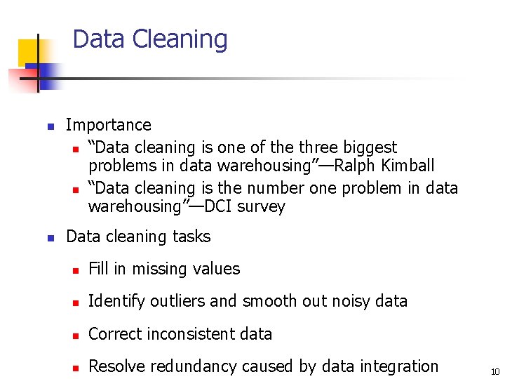
Data Cleaning n n Importance n “Data cleaning is one of the three biggest problems in data warehousing”—Ralph Kimball n “Data cleaning is the number one problem in data warehousing”—DCI survey Data cleaning tasks n Fill in missing values n Identify outliers and smooth out noisy data n Correct inconsistent data n Resolve redundancy caused by data integration 10

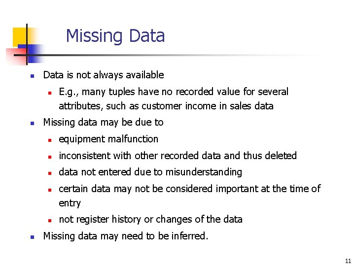
Missing Data n Data is not always available n n Missing data may be due to n equipment malfunction n inconsistent with other recorded data and thus deleted n data not entered due to misunderstanding n n n E. g. , many tuples have no recorded value for several attributes, such as customer income in sales data certain data may not be considered important at the time of entry not register history or changes of the data Missing data may need to be inferred. 11

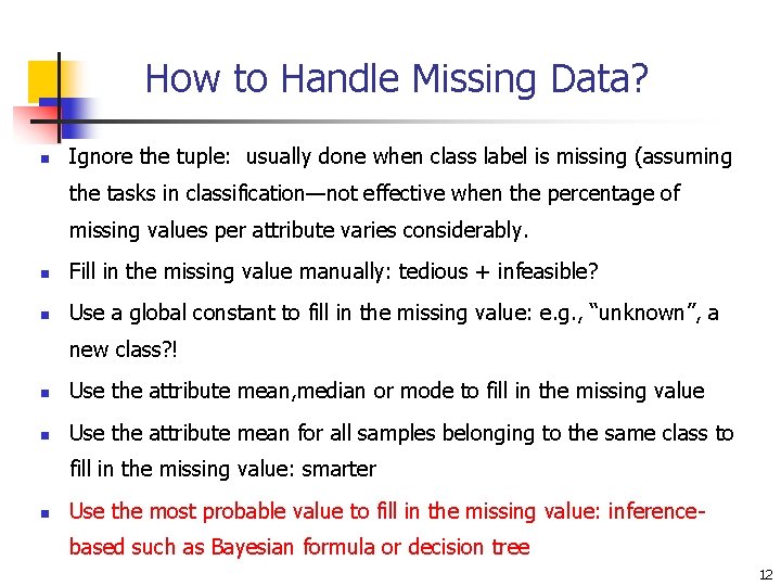
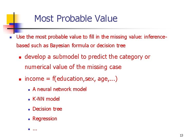
How to Handle Missing Data? n Ignore the tuple: usually done when class label is missing (assuming the tasks in classification—not effective when the percentage of missing values per attribute varies considerably. n Fill in the missing value manually: tedious + infeasible? n Use a global constant to fill in the missing value: e. g. , “unknown”, a new class? ! n Use the attribute mean, median or mode to fill in the missing value n Use the attribute mean for all samples belonging to the same class to fill in the missing value: smarter n Use the most probable value to fill in the missing value: inferencebased such as Bayesian formula or decision tree 12

Most Probable Value n Use the most probable value to fill in the missing value: inferencebased such as Bayesian formula or decision tree n develop a submodel to predict the category or numerical value of the missing case n income = f(education, sex, age, . . . ) n A neural network model n K-NN model n Decision tree n Regression n . . . 13

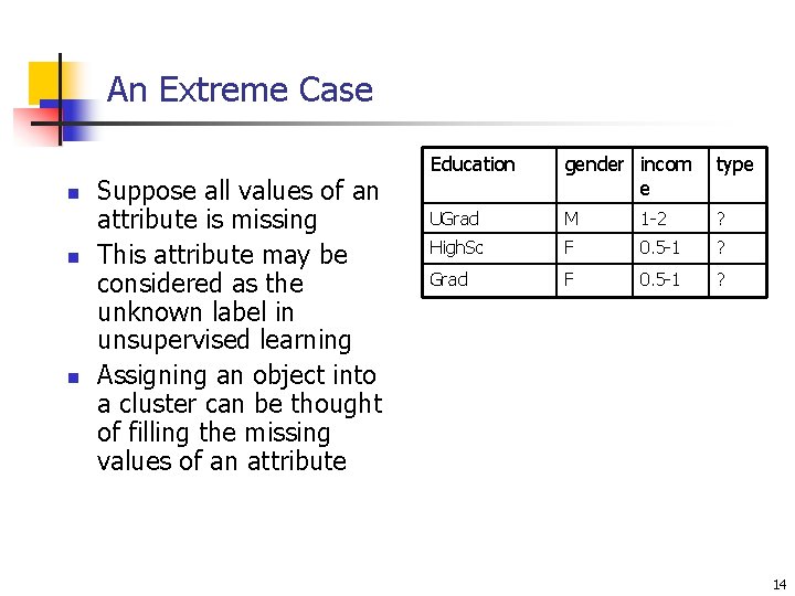
An Extreme Case n n n Suppose all values of an attribute is missing This attribute may be considered as the unknown label in unsupervised learning Assigning an object into a cluster can be thought of filling the missing values of an attribute Education gender incom e type UGrad M 1 -2 ? High. Sc F 0. 5 -1 ? Grad F 0. 5 -1 ? 14

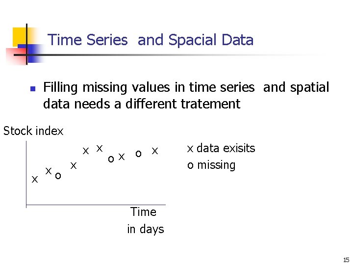
Time Series and Spacial Data n Filling missing values in time series and spatial data needs a different tratement Stock index x xo x x o x data exisits o missing Time in days 15

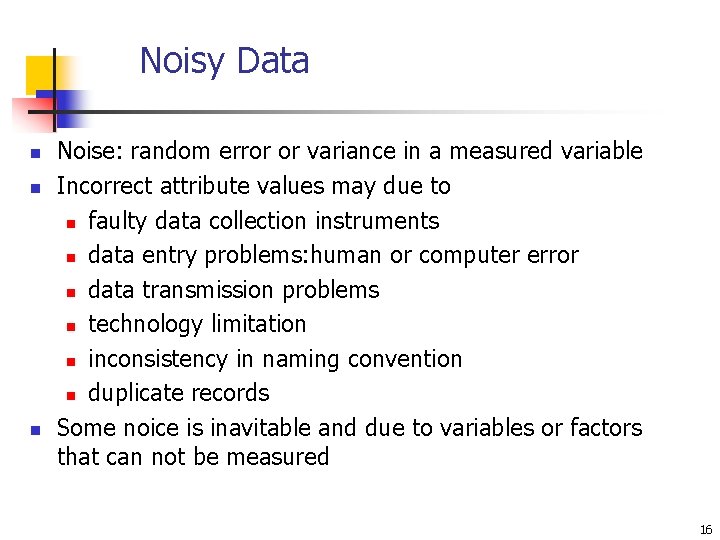
Noisy Data n n n Noise: random error or variance in a measured variable Incorrect attribute values may due to n faulty data collection instruments n data entry problems: human or computer error n data transmission problems n technology limitation n inconsistency in naming convention n duplicate records Some noice is inavitable and due to variables or factors that can not be measured 16

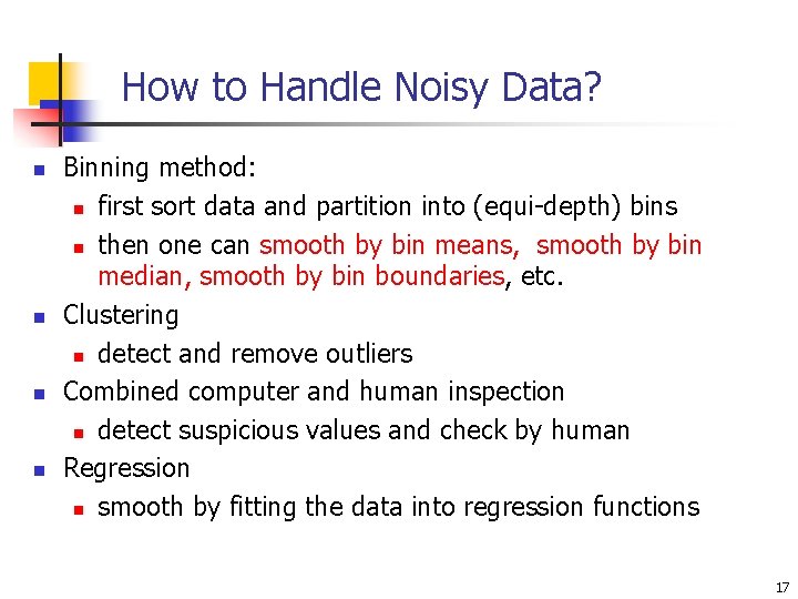
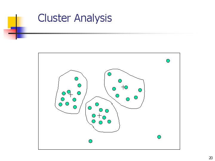
How to Handle Noisy Data? n n Binning method: n first sort data and partition into (equi-depth) bins n then one can smooth by bin means, smooth by bin median, smooth by bin boundaries, etc. Clustering n detect and remove outliers Combined computer and human inspection n detect suspicious values and check by human Regression n smooth by fitting the data into regression functions 17

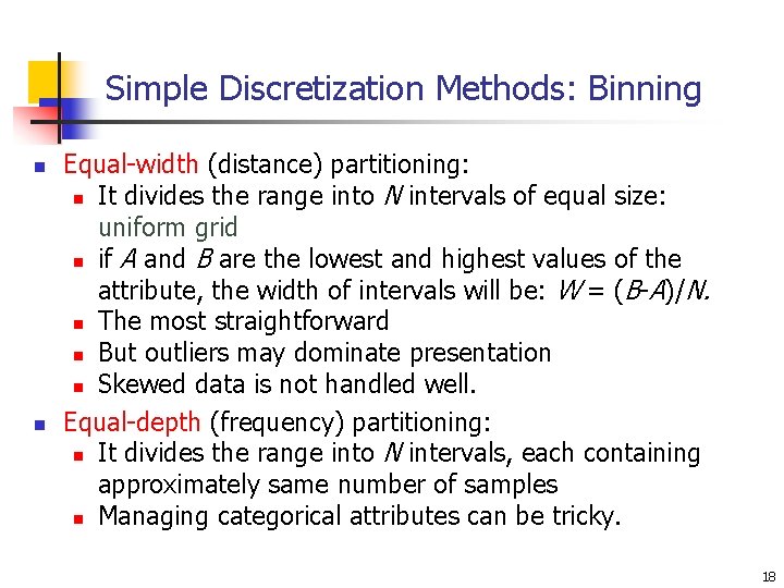
Simple Discretization Methods: Binning n n Equal-width (distance) partitioning: n It divides the range into N intervals of equal size: uniform grid n if A and B are the lowest and highest values of the attribute, the width of intervals will be: W = (B-A)/N. n The most straightforward n But outliers may dominate presentation n Skewed data is not handled well. Equal-depth (frequency) partitioning: n It divides the range into N intervals, each containing approximately same number of samples n Managing categorical attributes can be tricky. 18

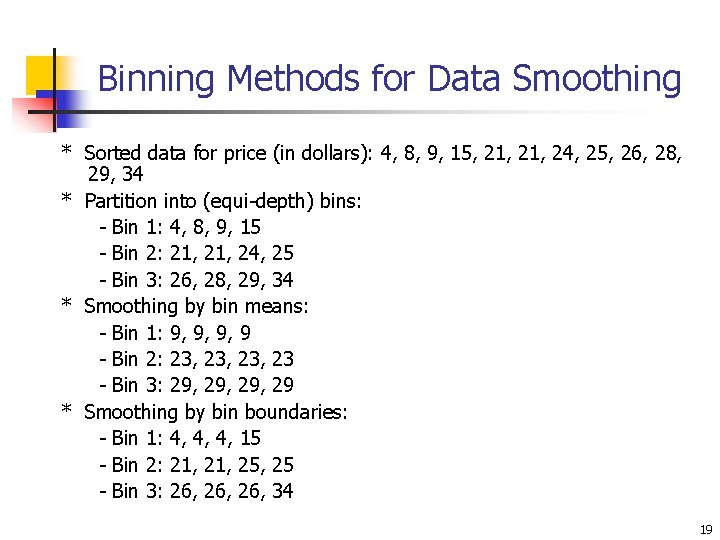
Binning Methods for Data Smoothing * Sorted data for price (in dollars): 4, 8, 9, 15, 21, 24, 25, 26, 28, 29, 34 * Partition into (equi-depth) bins: - Bin 1: 4, 8, 9, 15 - Bin 2: 21, 24, 25 - Bin 3: 26, 28, 29, 34 * Smoothing by bin means: - Bin 1: 9, 9, 9, 9 - Bin 2: 23, 23, 23 - Bin 3: 29, 29, 29 * Smoothing by bin boundaries: - Bin 1: 4, 4, 4, 15 - Bin 2: 21, 25, 25 - Bin 3: 26, 26, 34 19

Cluster Analysis 20

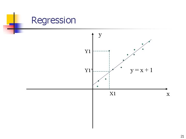
Regression y Y 1 y=x+1 Y 1’ X 1 x 21

Example use of regression to determine outliers n Problem: predict the yearly spending of AE customers from their income. n Y: yearly spending in YTL n X: average montly income in YTL 22

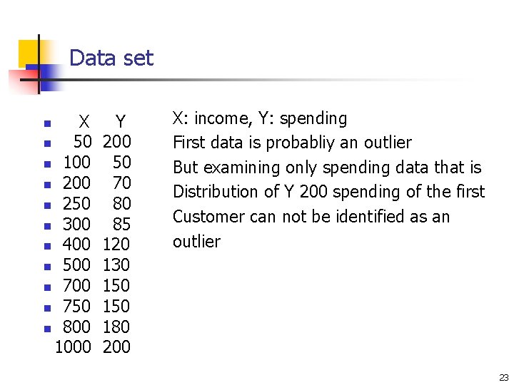
Data set X n 50 n 100 n 250 n 300 n 400 n 500 n 750 n 800 1000 n Y 200 50 70 80 85 120 130 150 180 200 X: income, Y: spending First data is probabliy an outlier But examining only spending data that is Distribution of Y 200 spending of the first Customer can not be identified as an outlier 23

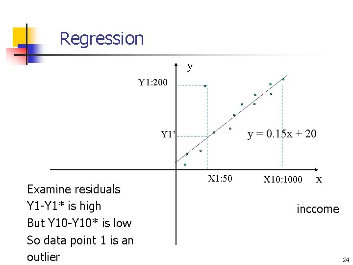
Regression y Y 1: 200 y = 0. 15 x + 20 Y 1’ Examine residuals Y 1 -Y 1* is high But Y 10 -Y 10* is low So data point 1 is an outlier X 1: 50 X 10: 1000 x inccome 24

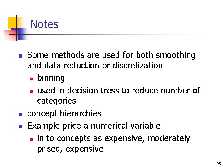
Notes n n n Some methods are used for both smoothing and data reduction or discretization n binning n used in decision tress to reduce number of categories concept hierarchies Example price a numerical variable n in to concepts as expensive, moderately prised, expensive 25

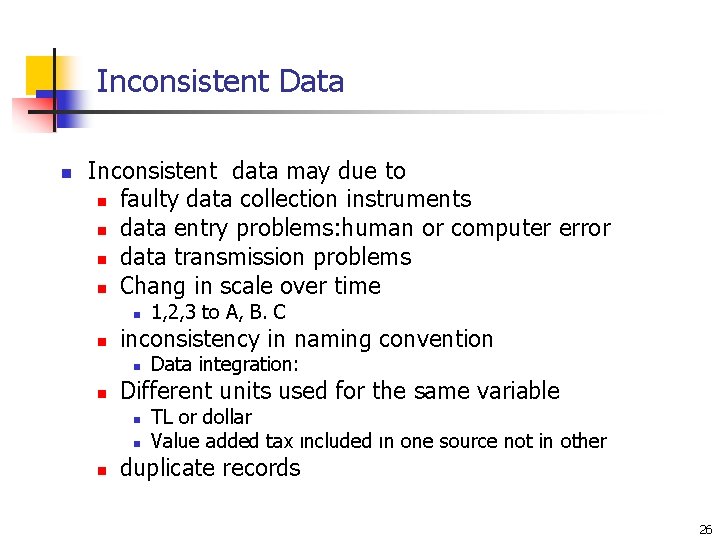
Inconsistent Data n Inconsistent data may due to n faulty data collection instruments n data entry problems: human or computer error n data transmission problems n Chang in scale over time n n inconsistency in naming convention n n Data integration: Different units used for the same variable n n n 1, 2, 3 to A, B. C TL or dollar Value added tax ıncluded ın one source not in other duplicate records 26

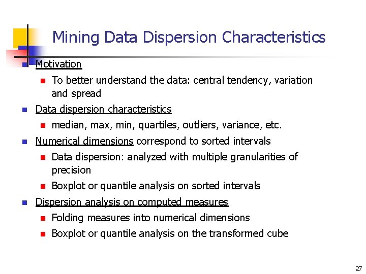
Mining Data Dispersion Characteristics n Motivation n n Data dispersion characteristics n n n To better understand the data: central tendency, variation and spread median, max, min, quartiles, outliers, variance, etc. Numerical dimensions correspond to sorted intervals n Data dispersion: analyzed with multiple granularities of precision n Boxplot or quantile analysis on sorted intervals Dispersion analysis on computed measures n Folding measures into numerical dimensions n Boxplot or quantile analysis on the transformed cube 27

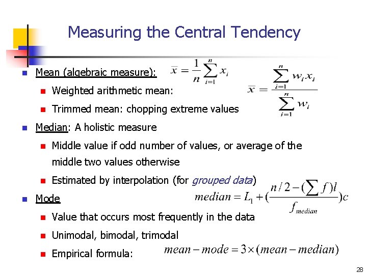
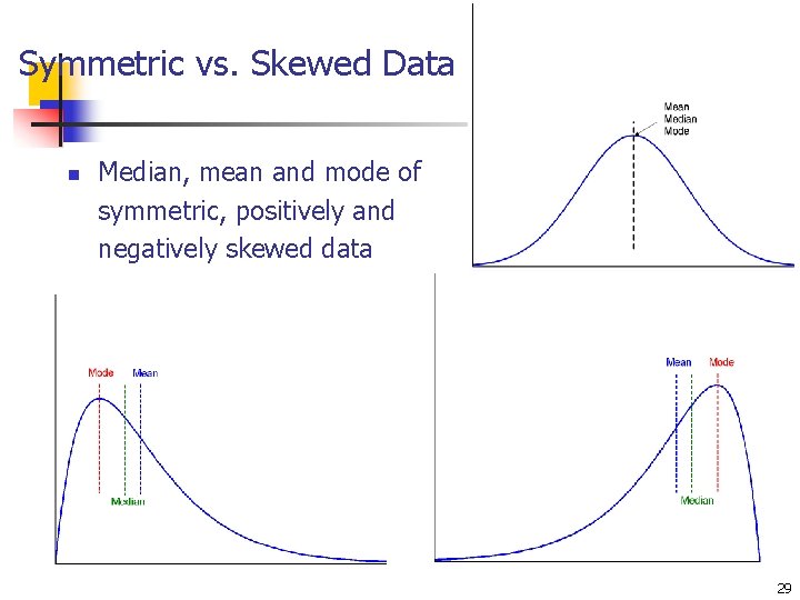
Measuring the Central Tendency n n Mean (algebraic measure): n Weighted arithmetic mean: n Trimmed mean: chopping extreme values Median: A holistic measure n Middle value if odd number of values, or average of the middle two values otherwise n n Estimated by interpolation (for grouped data) Mode n Value that occurs most frequently in the data n Unimodal, bimodal, trimodal n Empirical formula: 28

Symmetric vs. Skewed Data n Median, mean and mode of symmetric, positively and negatively skewed data 29

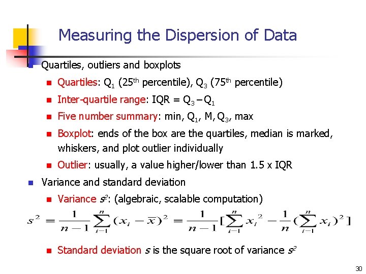
Measuring the Dispersion of Data n n Quartiles, outliers and boxplots n Quartiles: Q 1 (25 th percentile), Q 3 (75 th percentile) n Inter-quartile range: IQR = Q 3 – Q 1 n Five number summary: min, Q 1, M, Q 3, max n Boxplot: ends of the box are the quartiles, median is marked, whiskers, and plot outlier individually n Outlier: usually, a value higher/lower than 1. 5 x IQR Variance and standard deviation n Variance s 2: (algebraic, scalable computation) n Standard deviation s is the square root of variance s 2 30

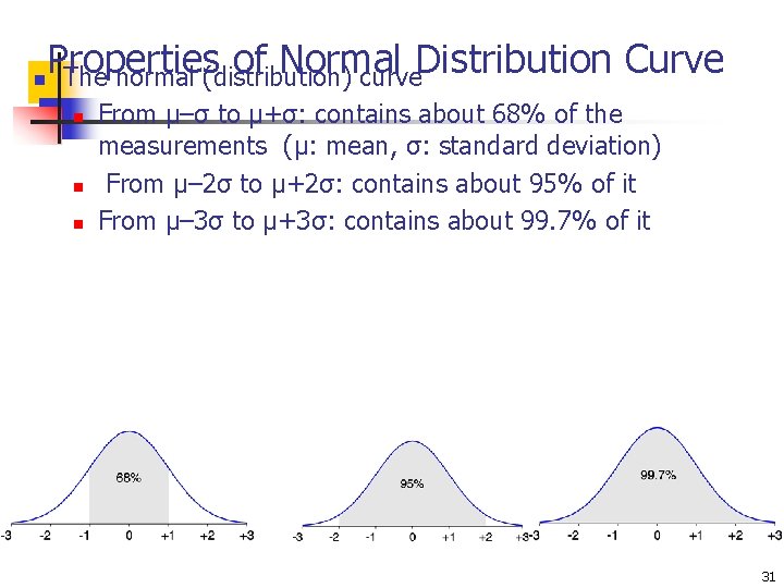
n Properties of Normal The normal (distribution) curve. Distribution Curve n n n From μ–σ to μ+σ: contains about 68% of the measurements (μ: mean, σ: standard deviation) From μ– 2σ to μ+2σ: contains about 95% of it From μ– 3σ to μ+3σ: contains about 99. 7% of it 31

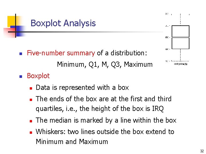
Boxplot Analysis n Five-number summary of a distribution: Minimum, Q 1, M, Q 3, Maximum n Boxplot n n Data is represented with a box The ends of the box are at the first and third quartiles, i. e. , the height of the box is IRQ The median is marked by a line within the box Whiskers: two lines outside the box extend to Minimum and Maximum 32

Positively and Negatively Correlated Data 33

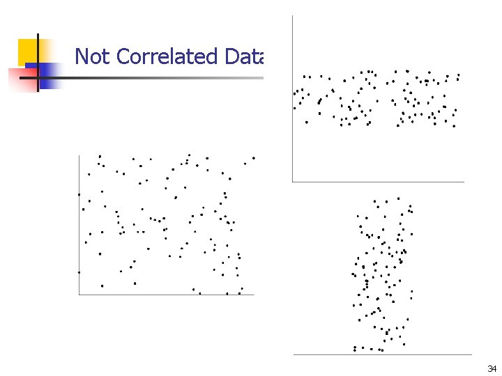
Not Correlated Data 34

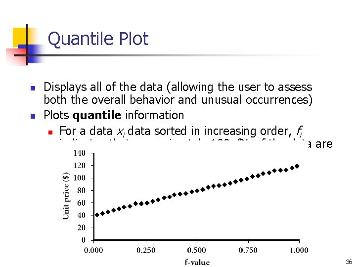
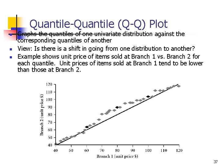
Graphic Displays of Basic Statistical Descriptions n n n Histogram: (shown before) Boxplot: (covered before) Quantile plot: each value xi is paired with fi indicating that approximately 100 fi % of data are xi Quantile-quantile (q-q) plot: graphs the quantiles of one univariant distribution against the corresponding quantiles of another Scatter plot: each pair of values is a pair of coordinates and plotted as points in the plane Loess (local regression) curve: add a smooth curve to a scatter plot to provide better perception of the pattern of dependence 35

Quantile Plot n n Displays all of the data (allowing the user to assess both the overall behavior and unusual occurrences) Plots quantile information n For a data xi data sorted in increasing order, fi indicates that approximately 100 fi% of the data are below or equal to the value xi Data Mining: Concepts and Techniques 36

Quantile-Quantile (Q-Q) Plot n n n Graphs the quantiles of one univariate distribution against the corresponding quantiles of another View: Is there is a shift in going from one distribution to another? Example shows unit price of items sold at Branch 1 vs. Branch 2 for each quantile. Unit prices of items sold at Branch 1 tend to be lower than those at Branch 2. 37

Chapter 3: Data Preprocessing n Why preprocess the data? n Data cleaning n Data integration and transformation n Data reduction n Discretization and concept hierarchy generation n Time-dependent data n Summary 38

Data Integration n Data integration: n combines data from multiple sources into a coherent store Schema integration n integrate metadata from different sources n Entity identification problem: identify real world entities from multiple data sources, e. g. , A. cust-id B. cust-# Detecting and resolving data value conflicts n for the same real world entity, attribute values from different sources are different n possible reasons: different representations, different scales, e. g. , metric vs. British units n price may include value added tax in one source and not include in the other n Name are entered by different convensıons: n name lastname or. . . 39

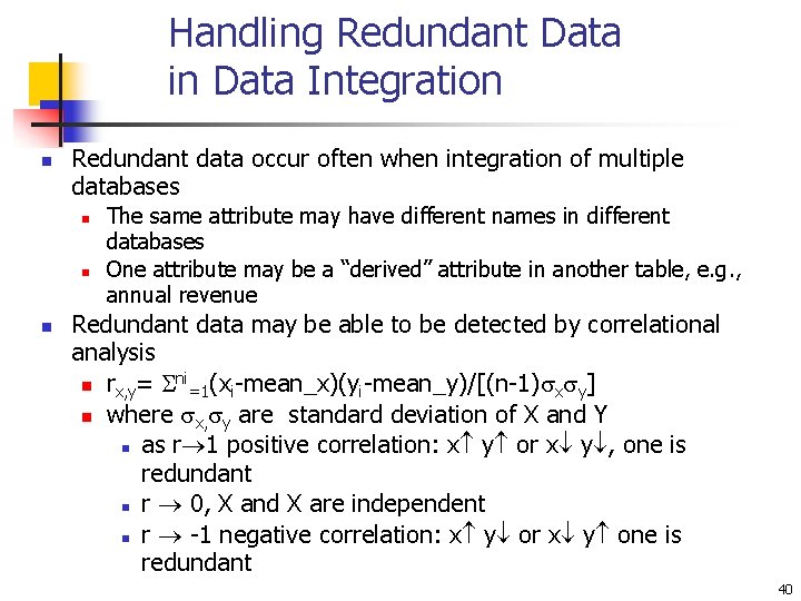
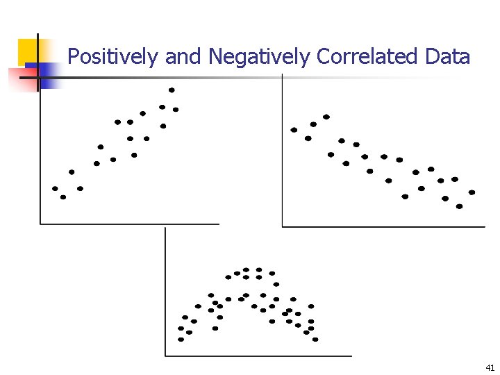
Handling Redundant Data in Data Integration n Redundant data occur often when integration of multiple databases n n n The same attribute may have different names in different databases One attribute may be a “derived” attribute in another table, e. g. , annual revenue Redundant data may be able to be detected by correlational analysis ni n rx, y= =1(xi-mean_x)(yi-mean_y)/[(n-1) x y] n where x, y are standard deviation of X and Y n as r 1 positive correlation: x y or x y , one is redundant n r 0, X and X are independent n r -1 negative correlation: x y or x y one is redundant 40

Positively and Negatively Correlated Data 41

Not Correlated Data 42

Exercise n n n Construct a data set or a functional relationship of two variables X and Y where there is a perfect relation between X and Y: n knowing value of X, Y corresponding to that X can be predicted with no error but correlation coefficient between X and Y is ZERO 43

Handling Redundant Data in Data Integration n how to detect redundancy for categorical variables? n n Find a measure of association for categorical variables Careful integration of the data from multiple sources may help reduce/avoid redundancies and inconsistencies and improve mining speed and quality 44

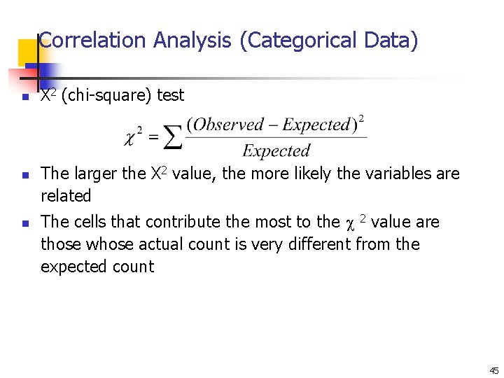
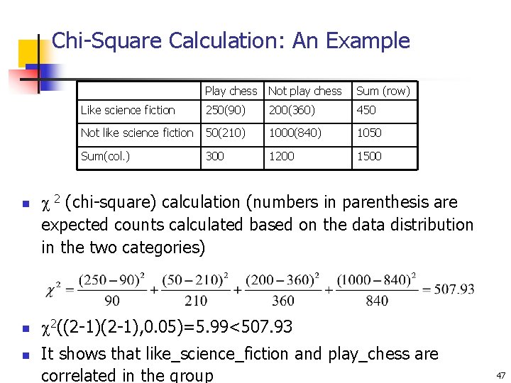
Correlation Analysis (Categorical Data) n n n Χ 2 (chi-square) test The larger the Χ 2 value, the more likely the variables are related The cells that contribute the most to the 2 value are those whose actual count is very different from the expected count 45

Chi-Square Test n Under the null hypothesis that attribute valuea are independent or not correlated 2 statistics is approximately distributed as n chi-square distribution with (k. A-1)*(k. B-1) degree of freedom n n n KA and KB are number of distinct values of attribute A and B Given a confidence level Reject null hypothesis of no correlation if 2 2 n > (df, ) 46

Chi-Square Calculation: An Example n n n Play chess Not play chess Sum (row) Like science fiction 250(90) 200(360) 450 Not like science fiction 50(210) 1000(840) 1050 Sum(col. ) 300 1200 1500 2 (chi-square) calculation (numbers in parenthesis are expected counts calculated based on the data distribution in the two categories) 2((2 -1), 0. 05)=5. 99<507. 93 It shows that like_science_fiction and play_chess are correlated in the group 47

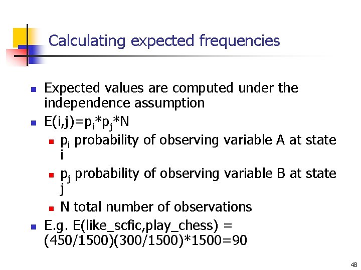
Calculating expected frequencies n n n Expected values are computed under the independence assumption E(i, j)=pi*pj*N n pi probability of observing variable A at state i n pj probability of observing variable B at state j n N total number of observations E. g. E(like_scfic, play_chess) = (450/1500)(300/1500)*1500=90 48

Exercises n n n What is the limitation of chi-square measure of correlation between categorical variables Suggest a better way of measuring correlation between categorical variables Suggest a way of measuring association between a categorical and a numerical variable 49

Correlation and Causation n Correlation does not imply causality n n # of hospitals and # of car-theft in a city are correlated Both are causally linked to the third variable: population 50

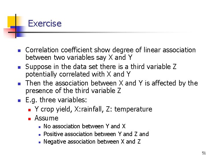
Exercise n n Correlation coefficient show degree of linear association between two variables say X and Y Suppose in the data set there is a third variable Z potentially correlated with X and Y Then the association between X and Y is affected by the presence of the third variable Z E. g. three variables: n Y crop yield, X: rainfall, Z: temperature n Assume n n n No association between Y and X Positive association between Y and Z and Negative association between X and Z 51

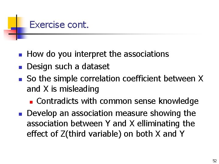
Exercise cont. n n How do you interpret the associations Design such a dataset So the simple correlation coefficient between X and X is misleading n Contradicts with common sense knowledge Develop an association measure showing the association between Y and X elliminating the effect of Z(third variable) on both X and Y 52

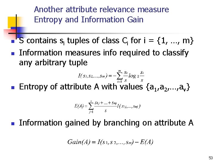
Another attribute relevance measure Entropy and Information Gain n S contains si tuples of class Ci for i = {1, …, m} Information measures info required to classify any arbitrary tuple n Entropy of attribute A with values {a 1, a 2, …, av} n Information gained by branching on attribute A n 53

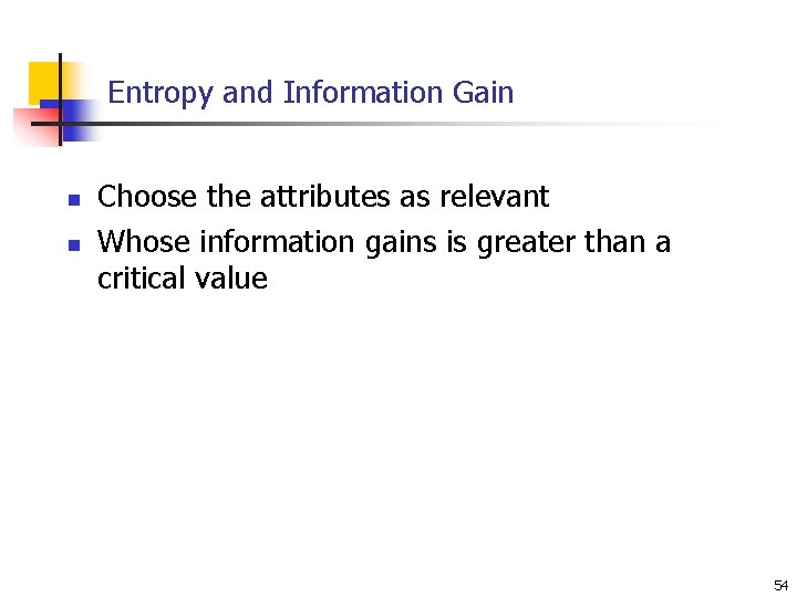
Entropy and Information Gain n n Choose the attributes as relevant Whose information gains is greater than a critical value 54

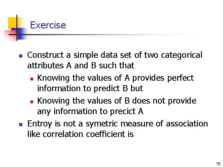
Exercise n n Construct a simple data set of two categorical attributes A and B such that n Knowing the values of A provides perfect information to predict B but n Knowing the values of B does not provide any information to precict A Entroy is not a symetric measure of association like correlation coefficient is 55

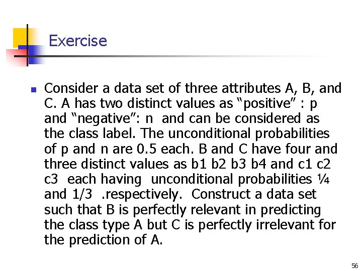
Exercise n Consider a data set of three attributes A, B, and C. A has two distinct values as “positive” : p and “negative”: n and can be considered as the class label. The unconditional probabilities of p and n are 0. 5 each. B and C have four and three distinct values as b 1 b 2 b 3 b 4 and c 1 c 2 c 3 each having unconditional probabilities ¼ and 1/3. respectively. Construct a data set such that B is perfectly relevant in predicting the class type A but C is perfectly irrelevant for the prediction of A. 56

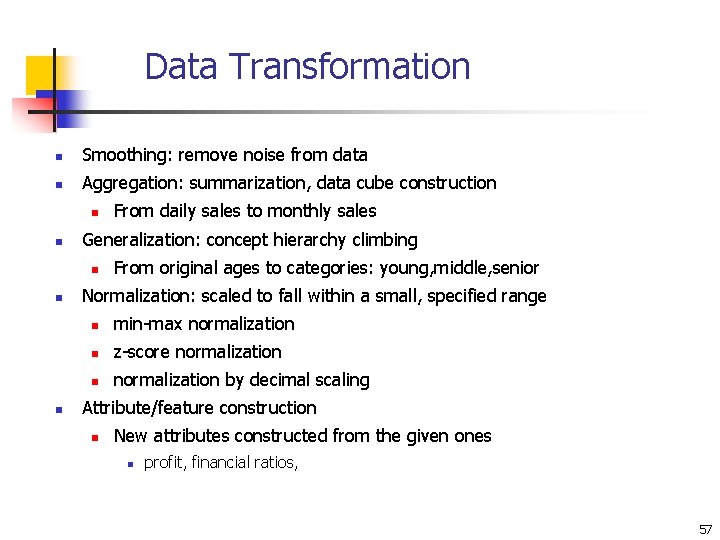
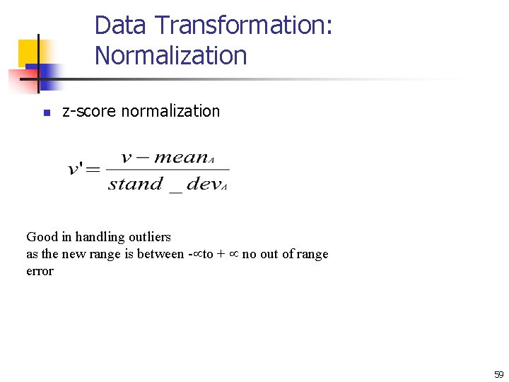
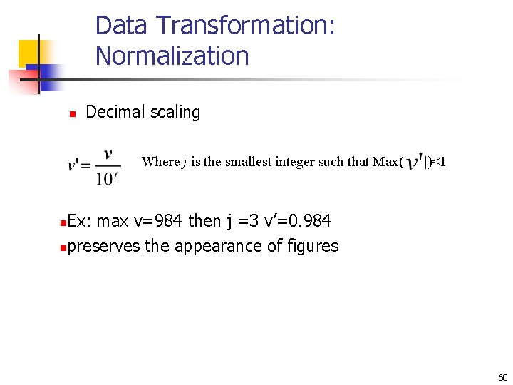
Data Transformation n Smoothing: remove noise from data n Aggregation: summarization, data cube construction n n Generalization: concept hierarchy climbing n n n From daily sales to monthly sales From original ages to categories: young, middle, senior Normalization: scaled to fall within a small, specified range n min-max normalization n z-score normalization n normalization by decimal scaling Attribute/feature construction n New attributes constructed from the given ones n profit, financial ratios, 57

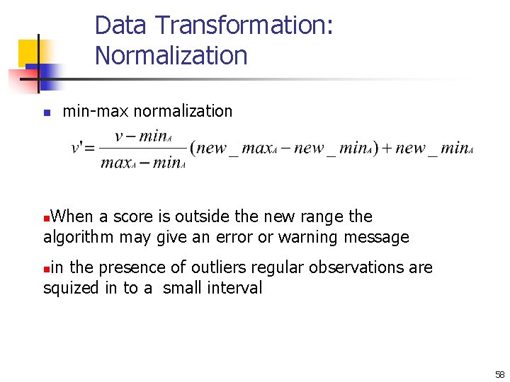
Data Transformation: Normalization n min-max normalization When a score is outside the new range the algorithm may give an error or warning message n in the presence of outliers regular observations are squized in to a small interval n 58

Data Transformation: Normalization n z-score normalization Good in handling outliers as the new range is between - to + no out of range error 59

Data Transformation: Normalization n Decimal scaling Where j is the smallest integer such that Max(| |)<1 Ex: max v=984 then j =3 v’=0. 984 npreserves the appearance of figures n 60

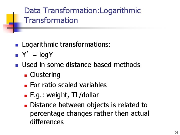
Data Transformation: Logarithmic Transformation n Logarithmic transformations: Y` = log. Y Used in some distance based methods n Clustering n For ratio scaled variables n E. g. : weight, TL/dollar n Distance between objects is related to percentage changes rather then actual differences 61

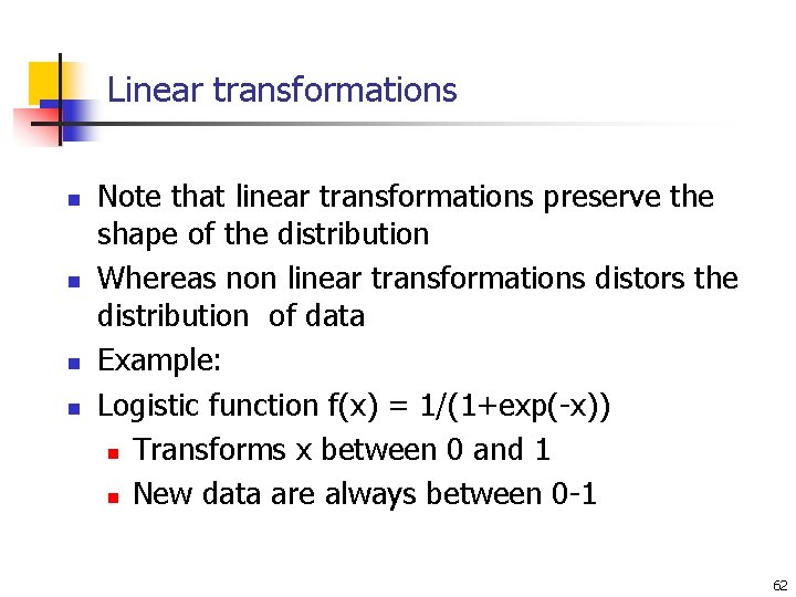
Linear transformations n n Note that linear transformations preserve the shape of the distribution Whereas non linear transformations distors the distribution of data Example: Logistic function f(x) = 1/(1+exp(-x)) n Transforms x between 0 and 1 n New data are always between 0 -1 62

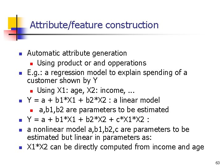
Attribute/feature construction n n n Automatic attribute generation n Using product or and opperations E. g. : a regression model to explain spending of a customer shown by Y n Using X 1: age, X 2: income, . . . Y = a + b 1*X 1 + b 2*X 2 : a linear model n a, b 1, b 2 are parameters to be estimated Y = a + b 1*X 1 + b 2*X 2 + c*X 1*X 2 : a nonlinear model a, b 1, b 2, c are parameters to be estimated but linear in parameters as: X 1*X 2 can be directly computed from income and age 63

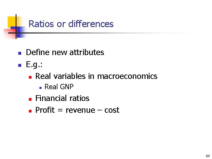
Ratios or differences n n Define new attributes E. g. : n Real variables in macroeconomics n n n Real GNP Financial ratios Profit = revenue – cost 64

Chapter 3: Data Preprocessing n Why preprocess the data? n Data cleaning n Data integration and transformation n Data reduction n Discretization and concept hierarchy generation n Time-dependent data n Summary 65

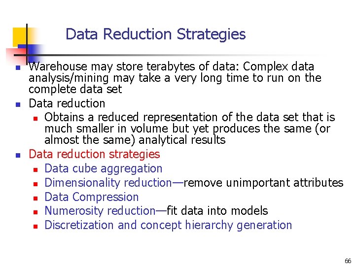
Data Reduction Strategies n n n Warehouse may store terabytes of data: Complex data analysis/mining may take a very long time to run on the complete data set Data reduction n Obtains a reduced representation of the data set that is much smaller in volume but yet produces the same (or almost the same) analytical results Data reduction strategies n Data cube aggregation n Dimensionality reduction—remove unimportant attributes n Data Compression n Numerosity reduction—fit data into models n Discretization and concept hierarchy generation 66

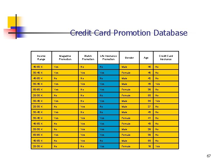
Credit Card Promotion Database Income Range Magazıne Promotıon Watch Promotıon Lıfe Insurance Promotıon Gender Credıt Card Insurance Age 40 -50 K Yes No No Male 45 No 30 -40 K Yes Yes Female 40 No 40 -50 K No No No Male 42 No 30 -40 K Yes Yes Male 43 Yes 50 -60 K Yes No Yes Female 38 No 20 -30 K No No No Female 55 No 30 -40 K Yes No Yes Male 35 Yes 20 -30 K No Yes No Male 27 No 30 -40 K Yes No No Male 43 No 30 -40 K Yes Yes Female 41 No 40 -50 K No Yes Female 43 No 20 -30 K No Yes Male 29 No 50 -60 K Yes Yes Female 39 No 40 -50 K No Yes No Male 55 No 20 -30 K No No Yes Female 19 Yes 67

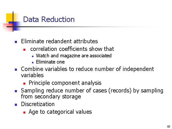
Data Reduction n Eliminate redandent attributes n correlation coefficients show that n n n Watch and magazine are associated Eliminate one Combine variables to reduce number of independent variables n Principle component analysis Sampling reduce number of cases (records) by sampling from secondary storage Discretization n Age to categorical values 68

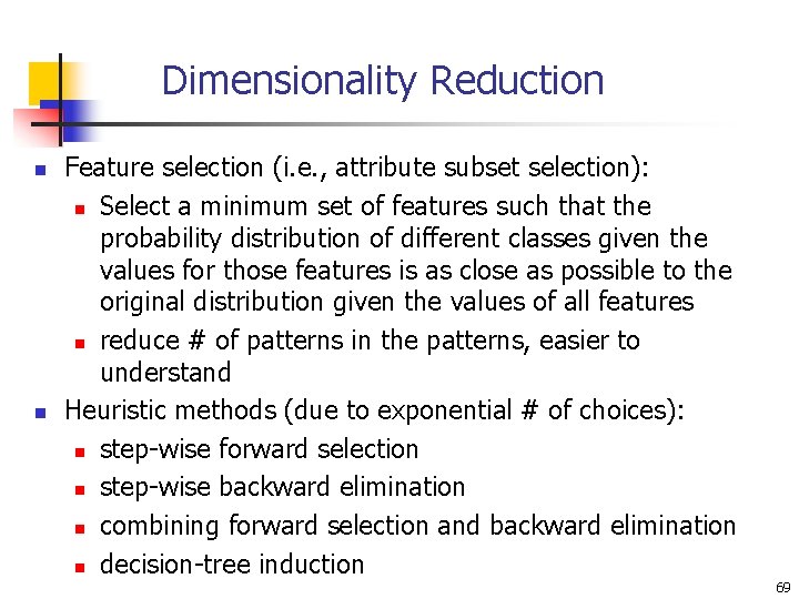
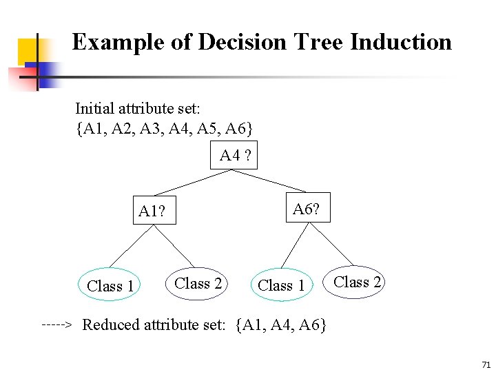
Dimensionality Reduction n n Feature selection (i. e. , attribute subset selection): n Select a minimum set of features such that the probability distribution of different classes given the values for those features is as close as possible to the original distribution given the values of all features n reduce # of patterns in the patterns, easier to understand Heuristic methods (due to exponential # of choices): n step-wise forward selection n step-wise backward elimination n combining forward selection and backward elimination n decision-tree induction 69

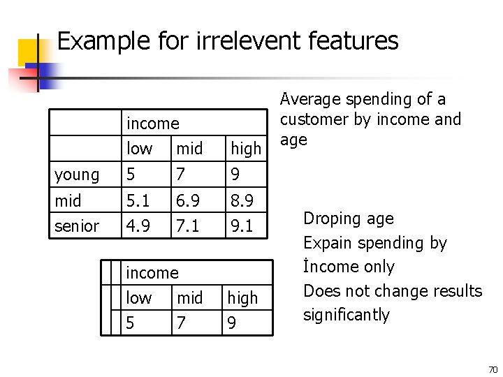
Example for irrelevent features income low mid high young 5 7 9 mid 5. 1 6. 9 8. 9 senior 4. 9 7. 1 9. 1 income low mid 5 7 high 9 Average spending of a customer by income and age Droping age Expain spending by İncome only Does not change results significantly 70

Example of Decision Tree Induction Initial attribute set: {A 1, A 2, A 3, A 4, A 5, A 6} A 4 ? A 6? A 1? Class 1 > Class 2 Class 1 Class 2 Reduced attribute set: {A 1, A 4, A 6} 71

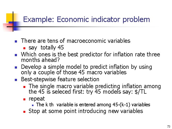
Example: Economic indicator problem n n There are tens of macroeconomic variables n say totally 45 Which ones is the best predictor for inflation rate three months ahead? Develop a simple model to predict inflation by using only a couple of those 45 macro variables Best-stepwise feature selection n The single macro variable predicting inflation among the 45 is seleced first: try 45 models say: $/TL n repeat n n The k th variable is entered among 45 -(k-1) variables Stop at some point introducing new variables 73

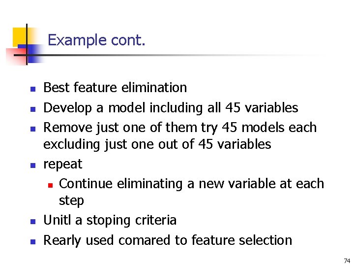
Example cont. n n n Best feature elimination Develop a model including all 45 variables Remove just one of them try 45 models each excluding just one out of 45 variables repeat n Continue eliminating a new variable at each step Unitl a stoping criteria Rearly used comared to feature selection 74

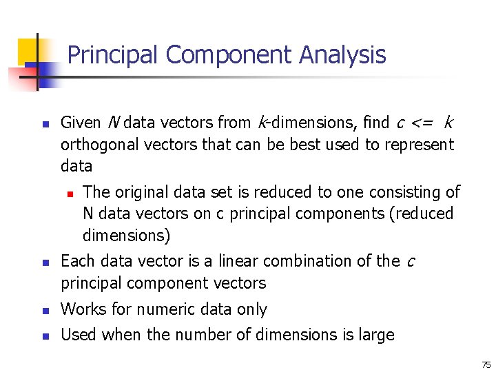
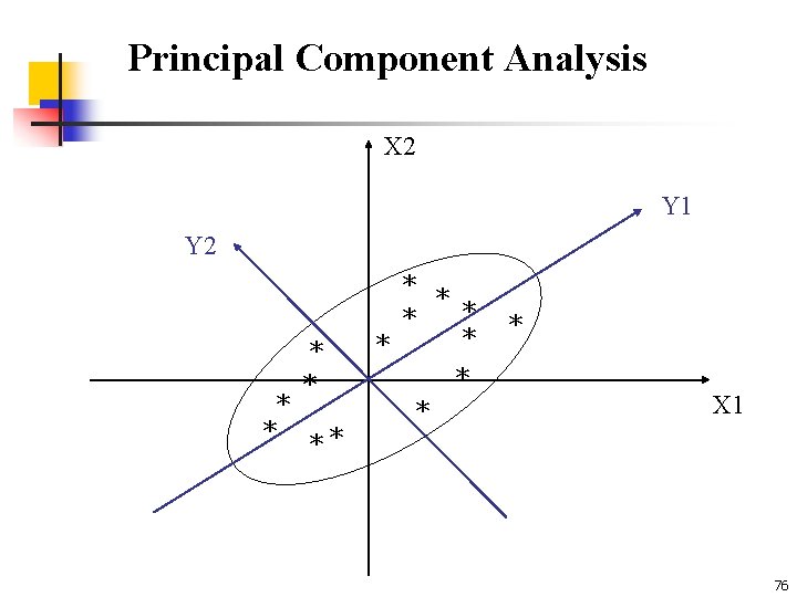
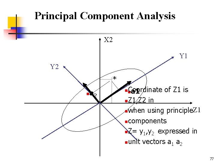
Principal Component Analysis n Given N data vectors from k-dimensions, find c <= k orthogonal vectors that can be best used to represent data n n The original data set is reduced to one consisting of N data vectors on c principal components (reduced dimensions) Each data vector is a linear combination of the c principal component vectors n Works for numeric data only n Used when the number of dimensions is large 75

Principal Component Analysis X 2 Y 1 Y 2 * * ** * * * * X 1 76

Principal Component Analysis X 2 Y 1 Y 2 * n a 2 Coordinate of Z 1 is a 1 n. Z 1, Z 2 in nwhen using principle. Z 1 ncomponents n. Z= y 1, y 2 expressed in nunit vectors a 1 a 2 nn 77

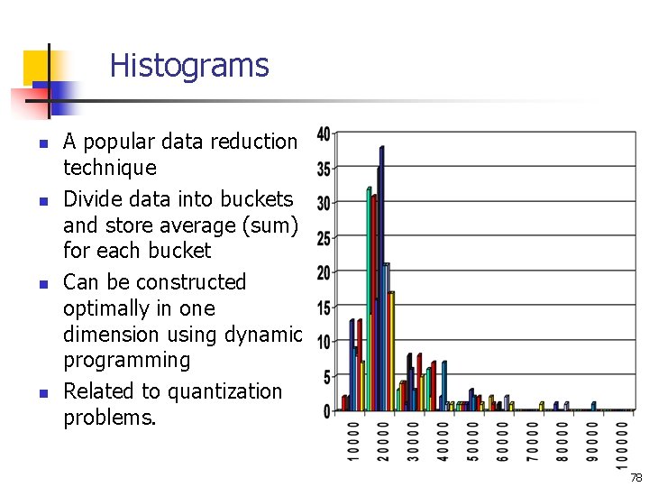
Histograms n n A popular data reduction technique Divide data into buckets and store average (sum) for each bucket Can be constructed optimally in one dimension using dynamic programming Related to quantization problems. 78

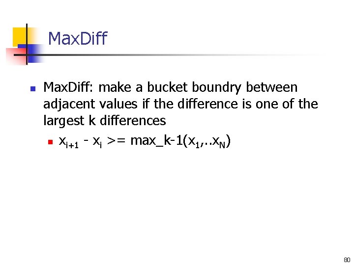
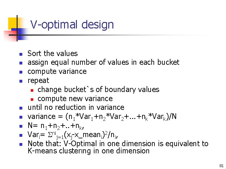
n n n Equiwidht: the width of each bucket range is uniform Equidepth (equiheight): each bucket contains roughly the same number of continuous data samples V-Optimal: least variance n histogram variance is the is a weighted sum of the original values that each bucket represents n bucket weight = #values in bucket 79

Max. Diff n Max. Diff: make a bucket boundry between adjacent values if the difference is one of the largest k differences n xi+1 - xi >= max_k-1(x 1, . . x. N) 80

V-optimal design n n n n Sort the values assign equal number of values in each bucket compute variance repeat n change bucket`s of boundary values n compute new variance until no reduction in variance = (n 1*Var 1+n 2*Var 2+. . . +nk*Vark)/N N= n 1+n 2+. . +nk, Vari= nij=1(xj-x_meani)2/ni, Note that: V-Optimal in one dimension is equivalent to K-means clusterıng in one dimension 81

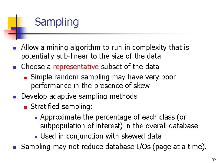
Sampling n n Allow a mining algorithm to run in complexity that is potentially sub-linear to the size of the data Choose a representative subset of the data n Simple random sampling may have very poor performance in the presence of skew Develop adaptive sampling methods n Stratified sampling: n Approximate the percentage of each class (or subpopulation of interest) in the overall database n Used in conjunction with skewed data Sampling may not reduce database I/Os (page at a time). 82

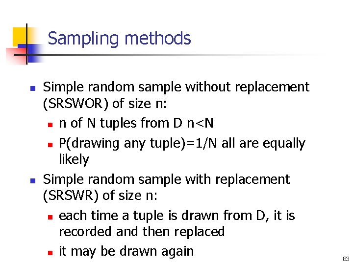
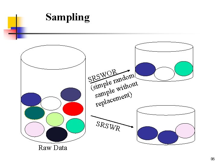
Sampling methods n n Simple random sample without replacement (SRSWOR) of size n: n n of N tuples from D n<N n P(drawing any tuple)=1/N all are equally likely Simple random sample with replacement (SRSWR) of size n: n each time a tuple is drawn from D, it is recorded and then replaced n it may be drawn again 83

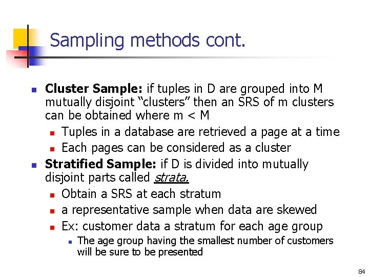
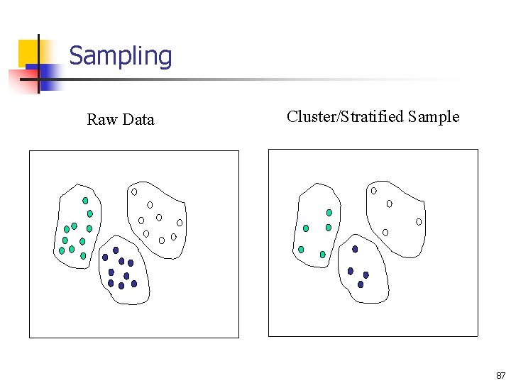
Sampling methods cont. n n Cluster Sample: if tuples in D are grouped into M mutually disjoint “clusters” then an SRS of m clusters can be obtained where m < M n Tuples in a database are retrieved a page at a time n Each pages can be considered as a cluster Stratified Sample: if D is divided into mutually disjoint parts called strata. n Obtain a SRS at each stratum n a representative sample when data are skewed n Ex: customer data a stratum for each age group n The age group having the smallest number of customers will be sure to be presented 84

Confidence intervals and sample size n n n Cost of obtaining a sample is propotional to the size of the sample, n Specifying a confidence interval and you should be able to determine n number of samples required so that the sample mean will be within the confidence interval with %(1 -p) confident n is very small compared to the size of the database N n<<N 85

Sampling R O W SRS le random t p u o m i h t s ( wi e l p sam ment) e c a l p re SRSW R Raw Data 86

Sampling Raw Data Cluster/Stratified Sample 87

Chapter 3: Data Preprocessing n Why preprocess the data? n Data cleaning n Data integration and transformation n Data reduction n Discretization and concept hierarchy generation n Time-dependent data n Summary 88

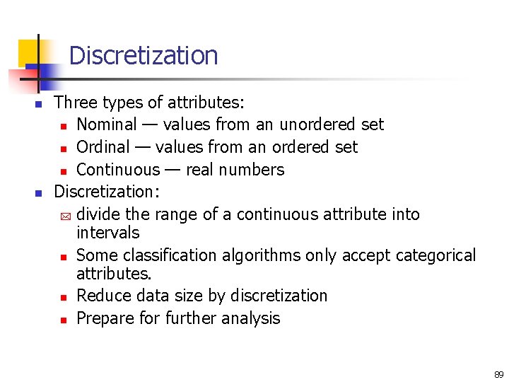
Discretization n n Three types of attributes: n Nominal — values from an unordered set n Ordinal — values from an ordered set n Continuous — real numbers Discretization: * divide the range of a continuous attribute into intervals n Some classification algorithms only accept categorical attributes. n Reduce data size by discretization n Prepare for further analysis 89

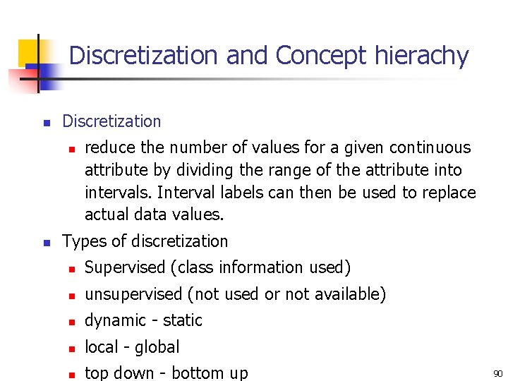
Discretization and Concept hierachy n Discretization n n reduce the number of values for a given continuous attribute by dividing the range of the attribute into intervals. Interval labels can then be used to replace actual data values. Types of discretization n Supervised (class information used) n unsupervised (not used or not available) n dynamic - static n local - global n top down - bottom up 90

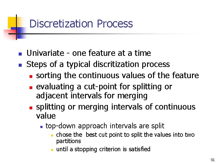
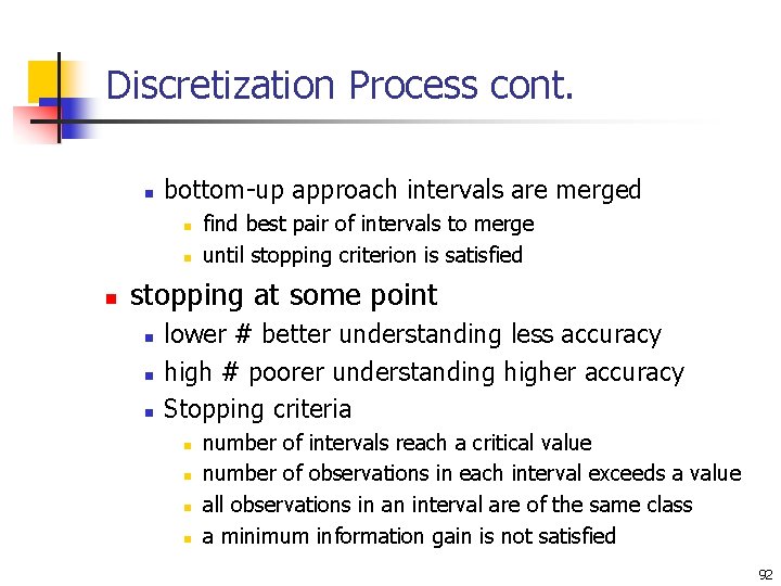
Discretization Process n n Univariate - one feature at a time Steps of a typical discritization process n sorting the continuous values of the feature n evaluating a cut-point for splitting or adjacent intervals for merging n splitting or merging intervals of continuous value n top-down approach intervals are split n n chose the best cut point to split the values into two partitions until a stopping criterion is satisfied 91

Discretization Process cont. n bottom-up approach intervals are merged n n n find best pair of intervals to merge until stopping criterion is satisfied stopping at some point n n n lower # better understanding less accuracy high # poorer understanding higher accuracy Stopping criteria n n number of intervals reach a critical value number of observations in each interval exceeds a value all observations in an interval are of the same class a minimum information gain is not satisfied 92

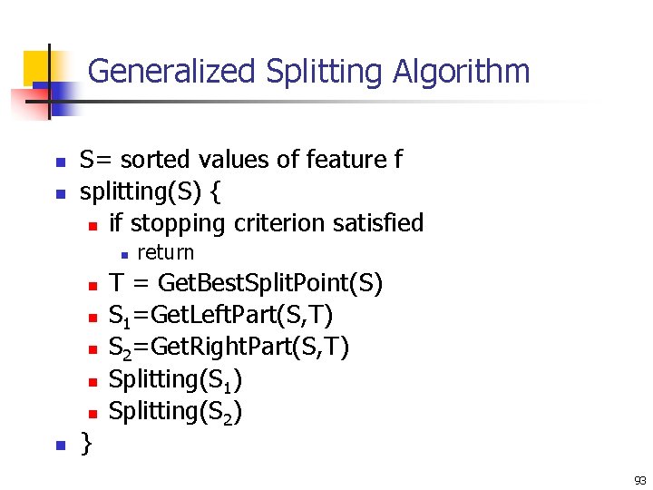
Generalized Splitting Algorithm n n S= sorted values of feature f splitting(S) { n if stopping criterion satisfied n n n n } return T = Get. Best. Split. Point(S) S 1=Get. Left. Part(S, T) S 2=Get. Right. Part(S, T) Splitting(S 1) Splitting(S 2) 93

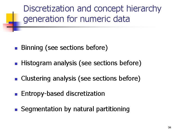
Discretization and concept hierarchy generation for numeric data n Binning (see sections before) n Histogram analysis (see sections before) n Clustering analysis (see sections before) n Entropy-based discretization n Segmentation by natural partitioning 94

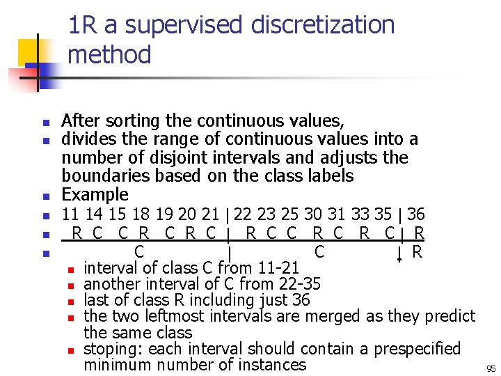
1 R a supervised discretization method n n n After sorting the continuous values, divides the range of continuous values into a number of disjoint intervals and adjusts the boundaries based on the class labels Example 11 14 15 18 19 20 21 22 23 25 30 31 33 35 36 R C C R C R C R C C R n interval of class C from 11 -21 n another interval of C from 22 -35 n last of class R including just 36 n the two leftmost intervals are merged as they predict the same class n stoping: each interval should contain a prespecified minimum number of instances 95

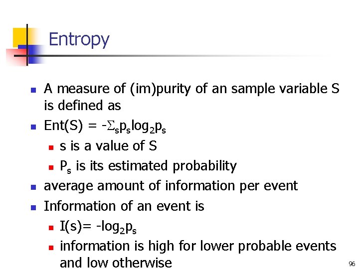
Entropy n n A measure of (im)purity of an sample variable S is defined as Ent(S) = - spslog 2 ps n s is a value of S n Ps is its estimated probability average amount of information per event Information of an event is n I(s)= -log 2 ps n information is high for lower probable events and low otherwise 96

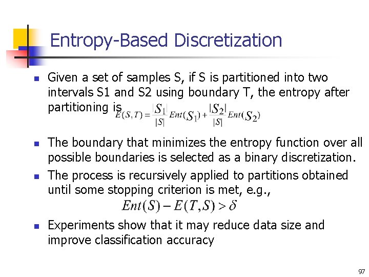
Entropy-Based Discretization n n Given a set of samples S, if S is partitioned into two intervals S 1 and S 2 using boundary T, the entropy after partitioning is The boundary that minimizes the entropy function over all possible boundaries is selected as a binary discretization. The process is recursively applied to partitions obtained until some stopping criterion is met, e. g. , Experiments show that it may reduce data size and improve classification accuracy 97

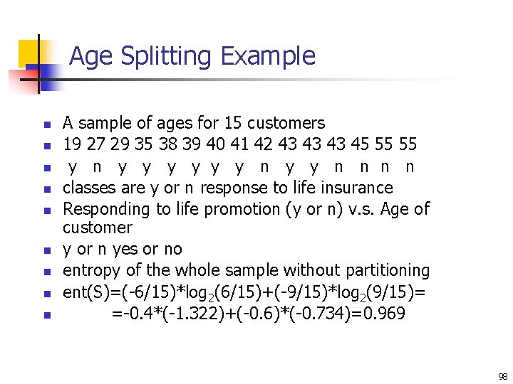
Age Splitting Example n n n n n A sample of ages for 15 customers 19 27 29 35 38 39 40 41 42 43 43 43 45 55 55 y n y y n n classes are y or n response to life insurance Responding to life promotion (y or n) v. s. Age of customer y or n yes or no entropy of the whole sample without partitioning ent(S)=(-6/15)*log 2(6/15)+(-9/15)*log 2(9/15)= =-0. 4*(-1. 322)+(-0. 6)*(-0. 734)=0. 969 98

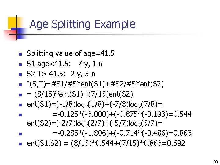
Age Splitting Example n n n n n Splitting value of age=41. 5 S 1 age<41. 5: 7 y, 1 n S 2 T> 41. 5: 2 y, 5 n I(S, T)=#S 1/#S*ent(S 1)+#S 2/#S*ent(S 2) = (8/15)*ent(S 1)+(7/15)ent(S 2) ent(S 1)=(-1/8)log 2(1/8)+(-7/8)log 2(7/8)= =-0. 125*(-3. 000)+(-0. 875*(-0. 193)=0. 544 ent(S 2)=(-2/7)log 2(2/7)+(-5/7)log 2(5/7)= =-0. 286*(-1. 806)+(-0. 714*(-0. 486)=0. 863 ent(S 1, S 2) = (8/15)*0. 544+(7/15)*0. 863=0. 692 99

Age Splitting Example n n n n Information gain: 0. 969 -0. 692=0. 277 try all possible partitions chose the partition providing maximum information gain then reccursively partition each interval until the stoping criteria is satisfied when information gain < a treshold value 100

Exercise 1. Consider a data set of two attributes A and B. A is continuous, whereas B is categorical, having two values as “y” and “n”, which can be considered as class of each observation. When attribute A is discretized into two equiwidth intervals no information is provided by the class attribute B but when discretized into three equiwidth intervals there is perfect information provided by B. Construct a simple dataset obeying these characteristics. 101