Data Transformations targeted at minimizing experimental variance n

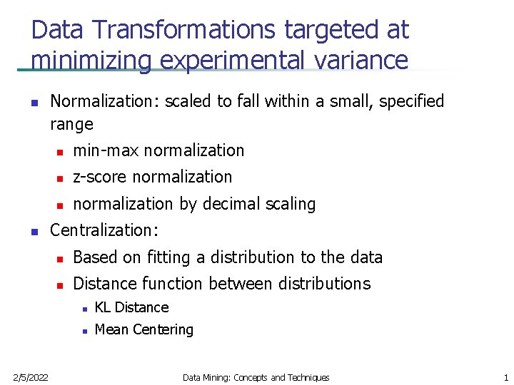
Data Transformations targeted at minimizing experimental variance n n 2/5/2022 Normalization: scaled to fall within a small, specified range n min-max normalization n z-score normalization n normalization by decimal scaling Centralization: n Based on fitting a distribution to the data n Distance function between distributions n KL Distance n Mean Centering Data Mining: Concepts and Techniques 1

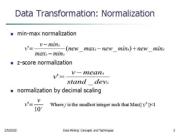
Data Transformation: Normalization n min-max normalization n z-score normalization n normalization by decimal scaling Where j is the smallest integer such that Max(| 2/5/2022 Data Mining: Concepts and Techniques |)<1 2

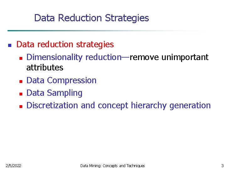
Data Reduction Strategies n Data reduction strategies n Dimensionality reduction—remove unimportant attributes n Data Compression n Data Sampling n Discretization and concept hierarchy generation 2/5/2022 Data Mining: Concepts and Techniques 3

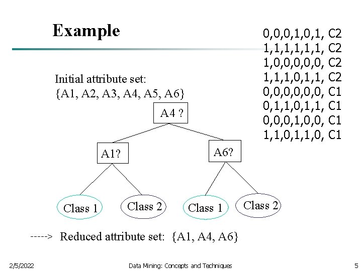
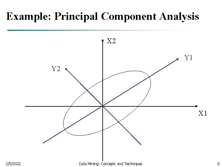
Dimensionality Reduction n n Feature selection (i. e. , attribute subset selection): n Set of possible solutions Power set n Heuristic search methods(due to exponential # of choices) n The goal is to identify the most useful subset of features for a given task, say classification. PCA: Given N data vectors from k-dimensions, find c <= k orthogonal vectors that can be best used to represent data n 2/5/2022 The original data set is reduced to one consisting of N data vectors on c principal components (reduced dimensions) Data Mining: Concepts and Techniques 4

Example 0, 0, 0, 1, 1, 1, 0, 0, 0, 1, 1, 1, 0, 0, 1, 1, 0, 0, 0, 1, 1, 0, Initial attribute set: {A 1, A 2, A 3, A 4, A 5, A 6} A 4 ? A 6? A 1? Class 1 > 2/5/2022 C 2 C 2 C 1 C 1 Class 2 Class 1 Class 2 Reduced attribute set: {A 1, A 4, A 6} Data Mining: Concepts and Techniques 5

Example: Principal Component Analysis X 2 Y 1 Y 2 X 1 2/5/2022 Data Mining: Concepts and Techniques 6

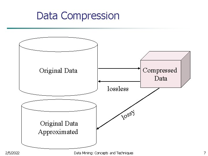
Data Compression Compressed Data Original Data lossless Original Data Approximated 2/5/2022 y s s lo Data Mining: Concepts and Techniques 7

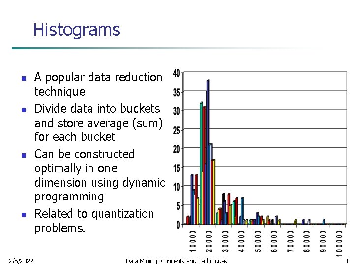
Histograms n n 2/5/2022 A popular data reduction technique Divide data into buckets and store average (sum) for each bucket Can be constructed optimally in one dimension using dynamic programming Related to quantization problems. Data Mining: Concepts and Techniques 8

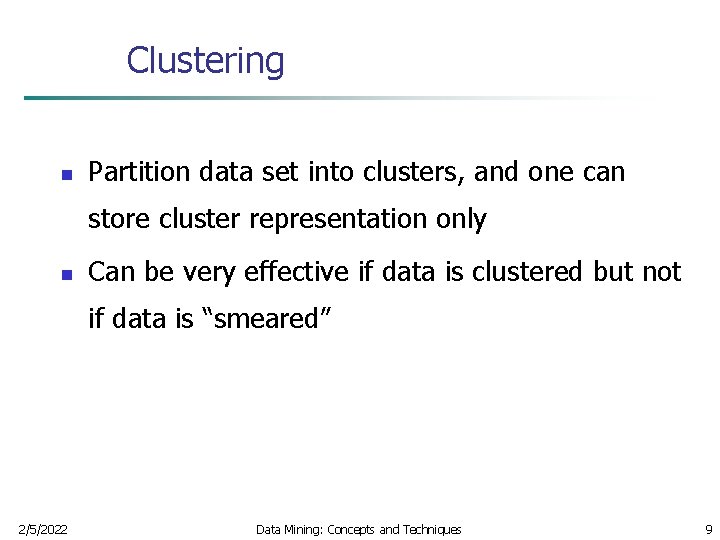
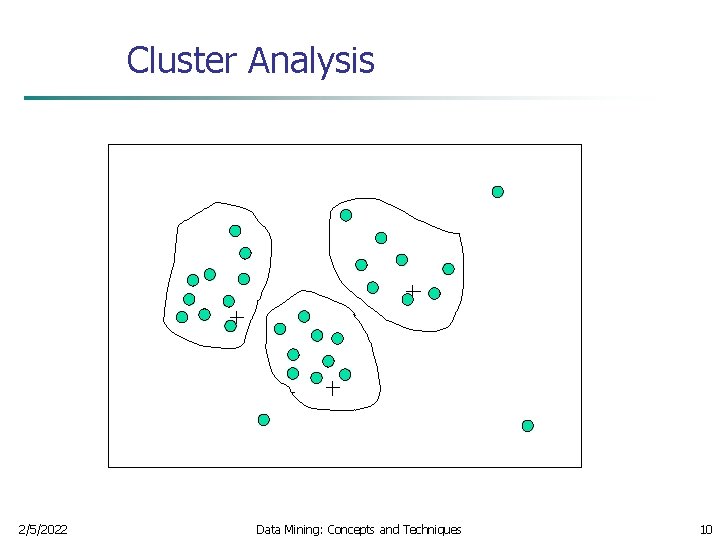
Clustering n Partition data set into clusters, and one can store cluster representation only n Can be very effective if data is clustered but not if data is “smeared” 2/5/2022 Data Mining: Concepts and Techniques 9

Cluster Analysis 2/5/2022 Data Mining: Concepts and Techniques 10

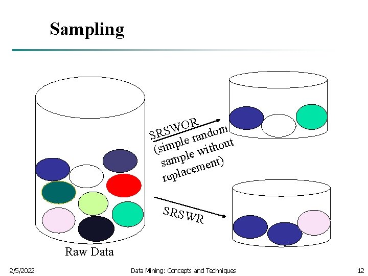
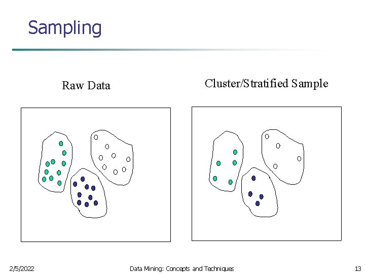
Sampling n n 2/5/2022 Allow a mining algorithm to run in complexity that is potentially sub-linear to the size of the data Choose a representative subset of the data n Simple random sampling may have very poor performance in the presence of skew Develop adaptive sampling methods n Stratified sampling: n Approximate the percentage of each class (or subpopulation of interest) in the overall database n Used in conjunction with skewed data Sampling may not reduce database I/Os (page at a time). Data Mining: Concepts and Techniques 11

Sampling R O W SRS le random t p u o m i h t s ( wi e l p sam ment) e c a l p re SRSW R Raw Data 2/5/2022 Data Mining: Concepts and Techniques 12

Sampling Raw Data 2/5/2022 Cluster/Stratified Sample Data Mining: Concepts and Techniques 13

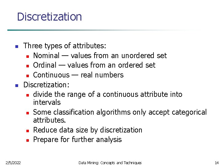
Discretization n n 2/5/2022 Three types of attributes: n Nominal — values from an unordered set n Ordinal — values from an ordered set n Continuous — real numbers Discretization: n divide the range of a continuous attribute into intervals n Some classification algorithms only accept categorical attributes. n Reduce data size by discretization n Prepare for further analysis Data Mining: Concepts and Techniques 14

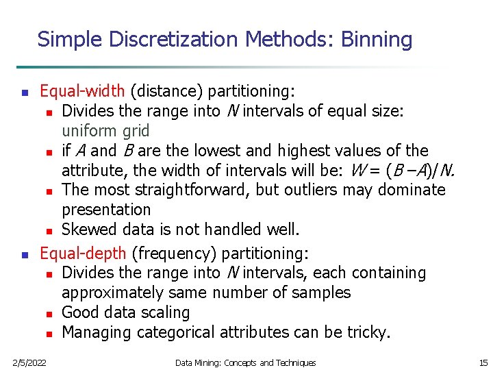
Simple Discretization Methods: Binning n n Equal-width (distance) partitioning: n Divides the range into N intervals of equal size: uniform grid n if A and B are the lowest and highest values of the attribute, the width of intervals will be: W = (B –A)/N. n The most straightforward, but outliers may dominate presentation n Skewed data is not handled well. Equal-depth (frequency) partitioning: n Divides the range into N intervals, each containing approximately same number of samples n Good data scaling n Managing categorical attributes can be tricky. 2/5/2022 Data Mining: Concepts and Techniques 15

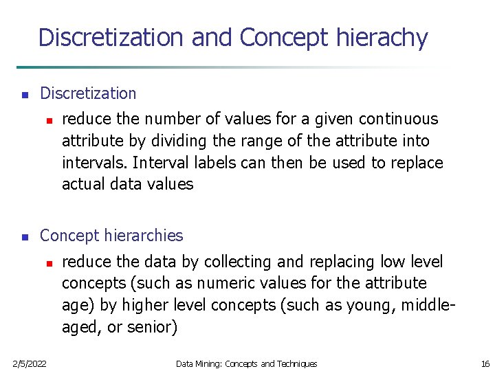
Discretization and Concept hierachy n Discretization n n reduce the number of values for a given continuous attribute by dividing the range of the attribute into intervals. Interval labels can then be used to replace actual data values Concept hierarchies n 2/5/2022 reduce the data by collecting and replacing low level concepts (such as numeric values for the attribute age) by higher level concepts (such as young, middleaged, or senior) Data Mining: Concepts and Techniques 16

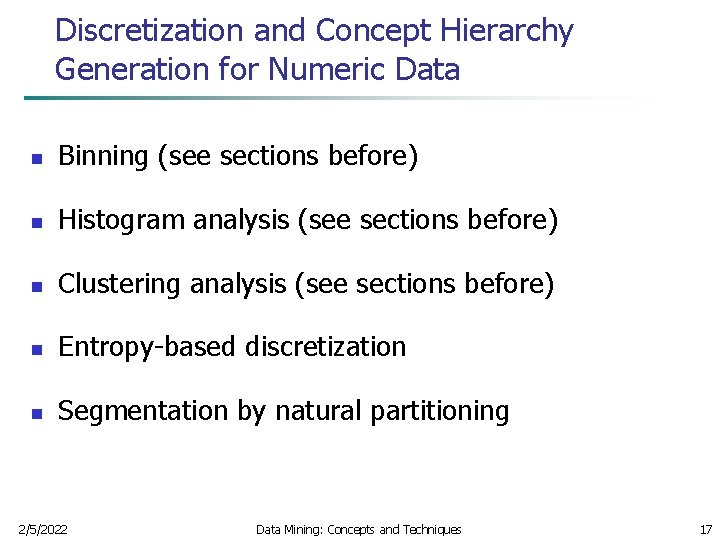
Discretization and Concept Hierarchy Generation for Numeric Data n Binning (see sections before) n Histogram analysis (see sections before) n Clustering analysis (see sections before) n Entropy-based discretization n Segmentation by natural partitioning 2/5/2022 Data Mining: Concepts and Techniques 17

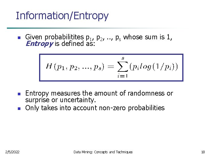
Information/Entropy n n n 2/5/2022 Given probabilitites p 1, p 2, . . , ps whose sum is 1, Entropy is defined as: Entropy measures the amount of randomness or surprise or uncertainty. Only takes into account non-zero probabilities Data Mining: Concepts and Techniques 18

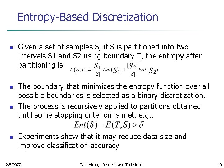
Entropy-Based Discretization n n Given a set of samples S, if S is partitioned into two intervals S 1 and S 2 using boundary T, the entropy after partitioning is The boundary that minimizes the entropy function over all possible boundaries is selected as a binary discretization. The process is recursively applied to partitions obtained until some stopping criterion is met, e. g. , Experiments show that it may reduce data size and improve classification accuracy 2/5/2022 Data Mining: Concepts and Techniques 19

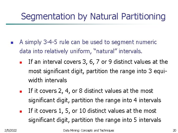
Segmentation by Natural Partitioning n A simply 3 -4 -5 rule can be used to segment numeric data into relatively uniform, “natural” intervals. n If an interval covers 3, 6, 7 or 9 distinct values at the most significant digit, partition the range into 3 equiwidth intervals n If it covers 2, 4, or 8 distinct values at the most significant digit, partition the range into 4 intervals n If it covers 1, 5, or 10 distinct values at the most significant digit, partition the range into 5 intervals 2/5/2022 Data Mining: Concepts and Techniques 20

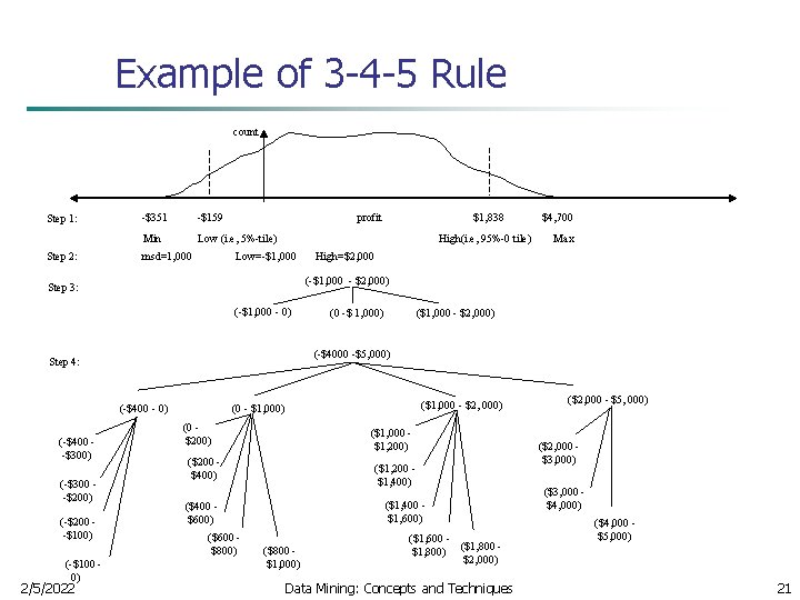
Example of 3 -4 -5 Rule count Step 1: Step 2: -$351 -$159 Min Low (i. e, 5%-tile) msd=1, 000 profit High(i. e, 95%-0 tile) Low=-$1, 000 (-$1, 000 - 0) (-$400 - 0) (-$200 -$100) (-$100 0) 2/5/2022 Max High=$2, 000 ($1, 000 - $2, 000) (0 -$ 1, 000) (-$4000 -$5, 000) Step 4: (-$300 -$200) $4, 700 (-$1, 000 - $2, 000) Step 3: (-$400 -$300) $1, 838 ($1, 000 - $2, 000) (0 - $1, 000) (0 $200) ($1, 000 $1, 200) ($200 $400) ($1, 200 $1, 400) ($1, 400 $1, 600) ($400 $600) ($600 $800) ($800 $1, 000) ($1, 600 ($1, 800) $2, 000) Data Mining: Concepts and Techniques ($2, 000 - $5, 000) ($2, 000 $3, 000) ($3, 000 $4, 000) ($4, 000 $5, 000) 21

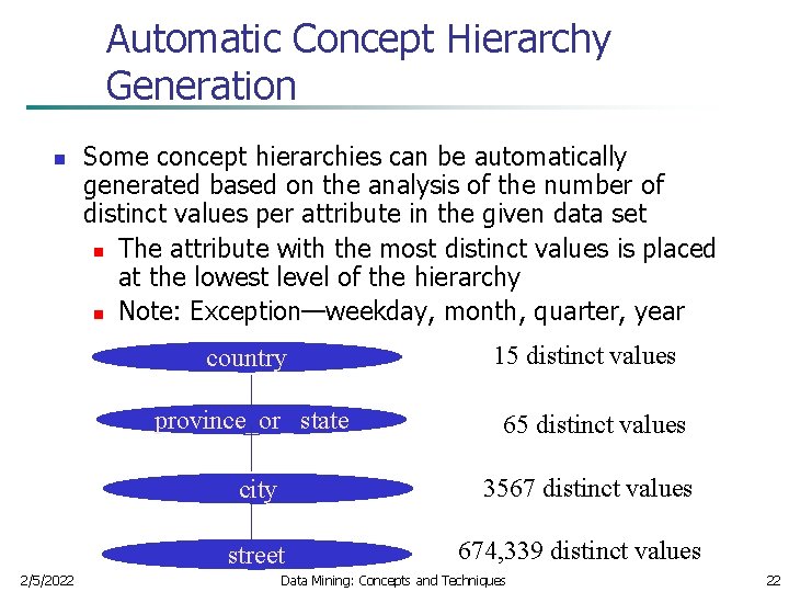
Automatic Concept Hierarchy Generation n Some concept hierarchies can be automatically generated based on the analysis of the number of distinct values per attribute in the given data set n The attribute with the most distinct values is placed at the lowest level of the hierarchy n Note: Exception—weekday, month, quarter, year country province_or_ state 65 distinct values city 3567 distinct values street 2/5/2022 15 distinct values 674, 339 distinct values Data Mining: Concepts and Techniques 22