Data Structures Unit1 Engineered for Tomorrow CSE MVJCE

Data Structures Unit-1 Engineered for Tomorrow CSE, MVJCE

Subject Name: Data Structures With C Subject Code: 10 CS 35 Prepared By: Alpana, Chandana, Sandhya, Sushma Department : CSE Date : 30/8/2014 CSC 2110 - Data Structures/Algorithms 2

Unit 1 Basic Concepts 1. 1 Pointers and Dynamic Memory Allocation 1. 2 Algorithm Specification 1. 3 Data Abstraction 1. 4 Performance Analysis 1. 5 Performance Measurement CSC 2110 - Data Structures/Algorithms 3

Pointers • Pointers – Powerful feature of the C++ language – One of the most difficult to master – Essential for construction of interesting data structures

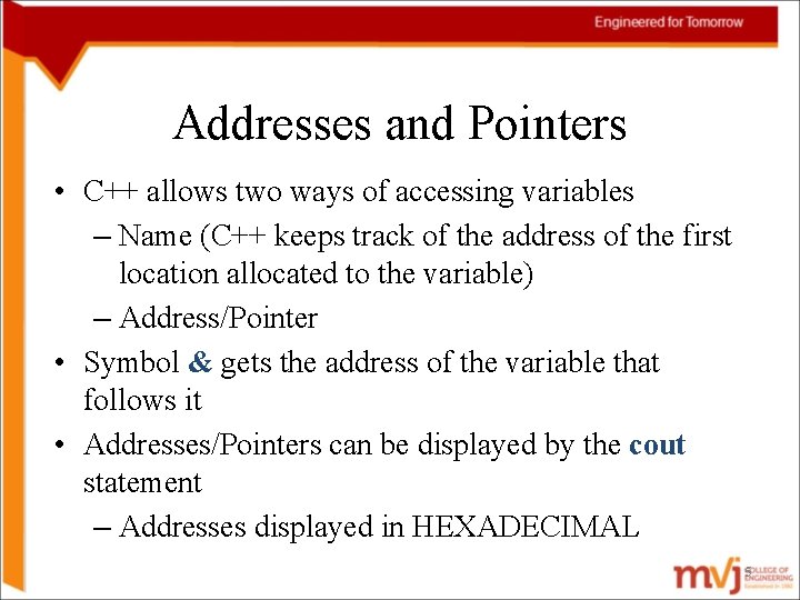
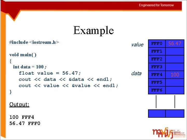
Addresses and Pointers • C++ allows two ways of accessing variables – Name (C++ keeps track of the address of the first location allocated to the variable) – Address/Pointer • Symbol & gets the address of the variable that follows it • Addresses/Pointers can be displayed by the cout statement – Addresses displayed in HEXADECIMAL 5

Example #include <iostream. h> void main( ) { int data = 100; float value = 56. 47; cout << data << &data << endl; cout << value << &value << endl; } value FFF 0 56. 47 FFF 1 FFF 2 FFF 3 data FFF 4 100 FFF 5 FFF 6 Output: 100 FFF 4 56. 47 FFF 0 6

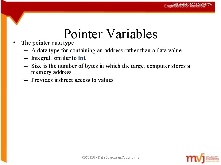
Engineered for Tomorrow • Pointer Variables The pointer data type – A data type for containing an address rather than a data value – Integral, similar to int – Size is the number of bytes in which the target computer stores a memory address – Provides indirect access to values CSC 2110 - Data Structures/Algorithms 7

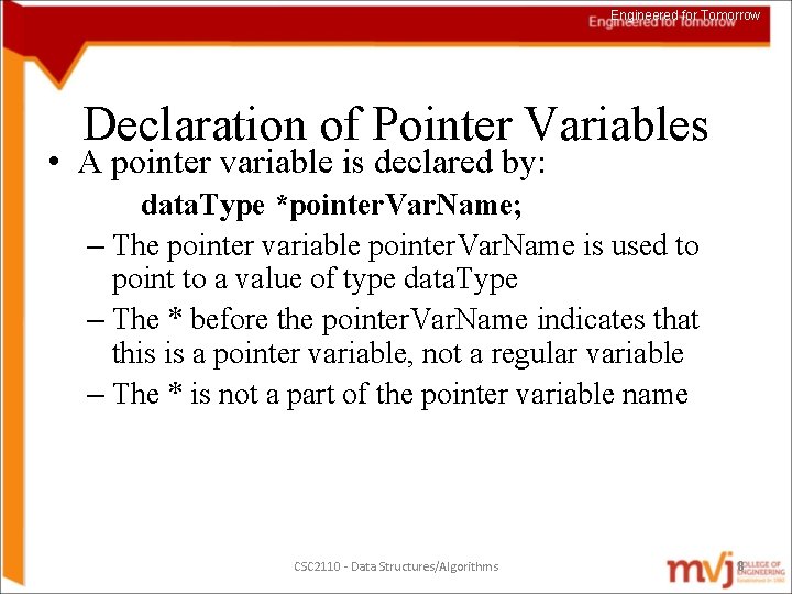
Engineered for Tomorrow Declaration of Pointer Variables • A pointer variable is declared by: data. Type *pointer. Var. Name; – The pointer variable pointer. Var. Name is used to point to a value of type data. Type – The * before the pointer. Var. Name indicates that this is a pointer variable, not a regular variable – The * is not a part of the pointer variable name CSC 2110 - Data Structures/Algorithms 8

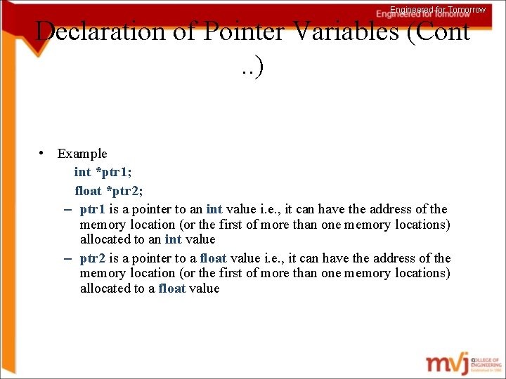
Engineered for Tomorrow Declaration of Pointer Variables (Cont. . ) • Example int *ptr 1; float *ptr 2; – ptr 1 is a pointer to an int value i. e. , it can have the address of the memory location (or the first of more than one memory locations) allocated to an int value – ptr 2 is a pointer to a float value i. e. , it can have the address of the memory location (or the first of more than one memory locations) allocated to a float value 9

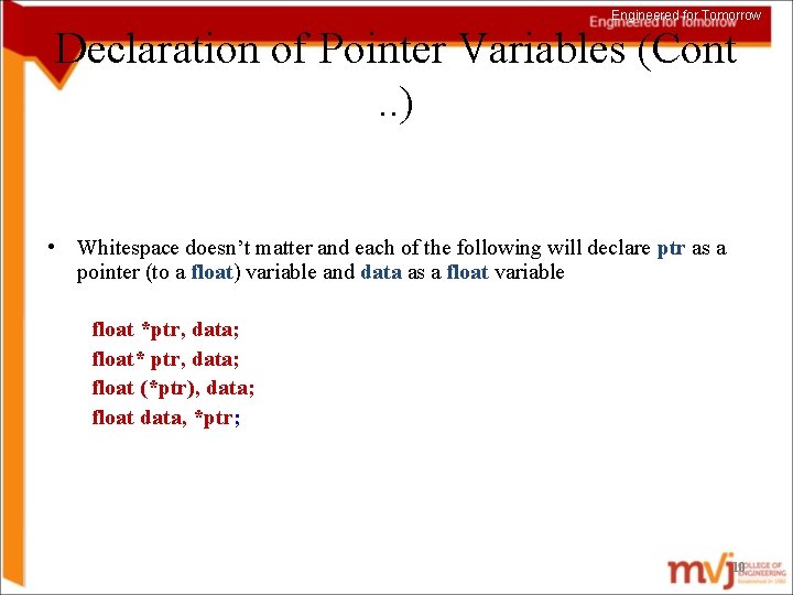
Engineered for Tomorrow Declaration of Pointer Variables (Cont. . ) • Whitespace doesn’t matter and each of the following will declare ptr as a pointer (to a float) variable and data as a float variable float *ptr, data; float* ptr, data; float (*ptr), data; float data, *ptr; 10

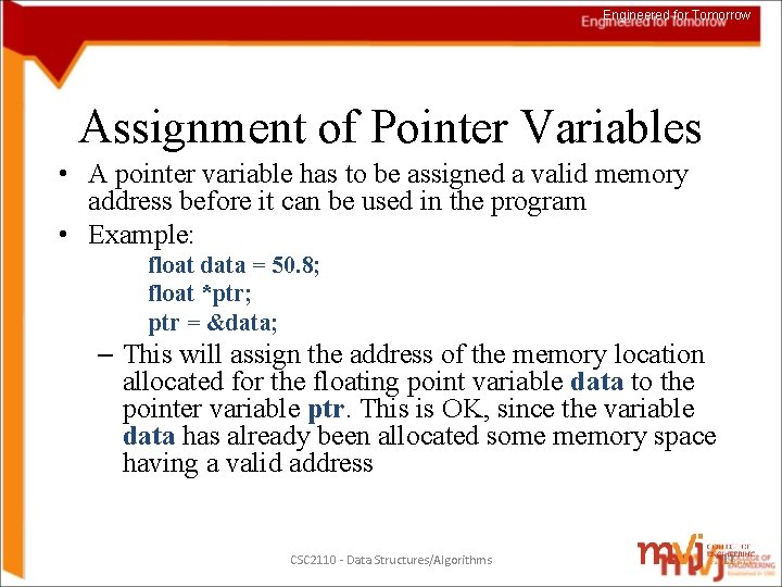
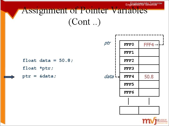
Engineered for Tomorrow Assignment of Pointer Variables • A pointer variable has to be assigned a valid memory address before it can be used in the program • Example: float data = 50. 8; float *ptr; ptr = &data; – This will assign the address of the memory location allocated for the floating point variable data to the pointer variable ptr. This is OK, since the variable data has already been allocated some memory space having a valid address CSC 2110 - Data Structures/Algorithms 11

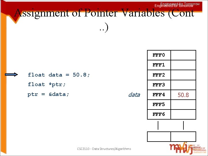
Engineered for Tomorrow Assignment of Pointer Variables (Cont. . ) FFF 0 FFF 1 float data = 50. 8; FFF 2 float *ptr; FFF 3 ptr = &data; data FFF 4 50. 8 FFF 5 FFF 6 CSC 2110 - Data Structures/Algorithms 12

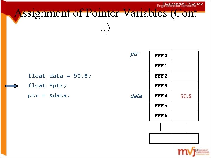
Engineered for Tomorrow Assignment of Pointer Variables (Cont. . ) ptr FFF 0 FFF 1 float data = 50. 8; FFF 2 float *ptr; FFF 3 ptr = &data; data FFF 4 50. 8 FFF 5 FFF 6 13

Engineered for Tomorrow Assignment of Pointer Variables (Cont. . ) ptr FFF 0 FFF 4 FFF 1 float data = 50. 8; FFF 2 float *ptr; FFF 3 ptr = &data; data FFF 4 50. 8 FFF 5 FFF 6 14

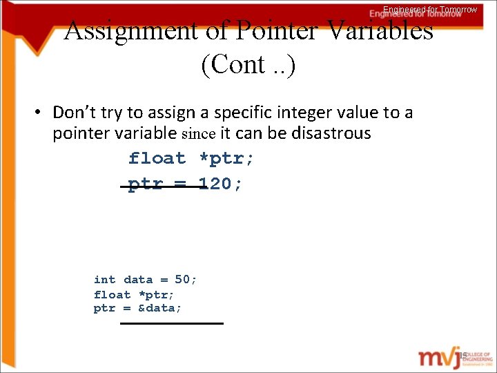
Engineered for Tomorrow Assignment of Pointer Variables (Cont. . ) • Don’t try to assign a specific integer value to a pointer variable since it can be disastrous float *ptr; ptr = 120; • You cannot assign the address of one type of variable to a pointer variable of another type even though they are both integrals int data = 50; float *ptr; ptr = &data; 15

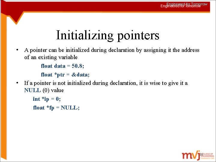
Engineered for Tomorrow Initializing pointers • A pointer can be initialized during declaration by assigning it the address of an existing variable float data = 50. 8; float *ptr = &data; • If a pointer is not initialized during declaration, it is wise to give it a NULL (0) value int *ip = 0; float *fp = NULL; 16

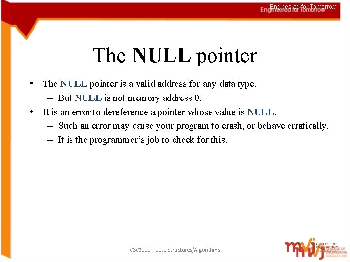
Engineered for Tomorrow The NULL pointer • The NULL pointer is a valid address for any data type. – But NULL is not memory address 0. • It is an error to dereference a pointer whose value is NULL. – Such an error may cause your program to crash, or behave erratically. – It is the programmer’s job to check for this. CSC 2110 - Data Structures/Algorithms 17

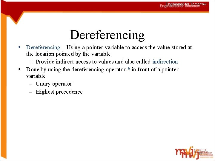
Engineered for Tomorrow Dereferencing • Dereferencing – Using a pointer variable to access the value stored at the location pointed by the variable – Provide indirect access to values and also called indirection • Done by using the dereferencing operator * in front of a pointer variable – Unary operator – Highest precedence 18

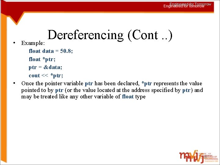
Engineered for Tomorrow • Dereferencing (Cont. . ) Example: float data = 50. 8; float *ptr; ptr = &data; cout << *ptr; • Once the pointer variable ptr has been declared, *ptr represents the value pointed to by ptr (or the value located at the address specified by ptr) and may be treated like any other variable of float type 19

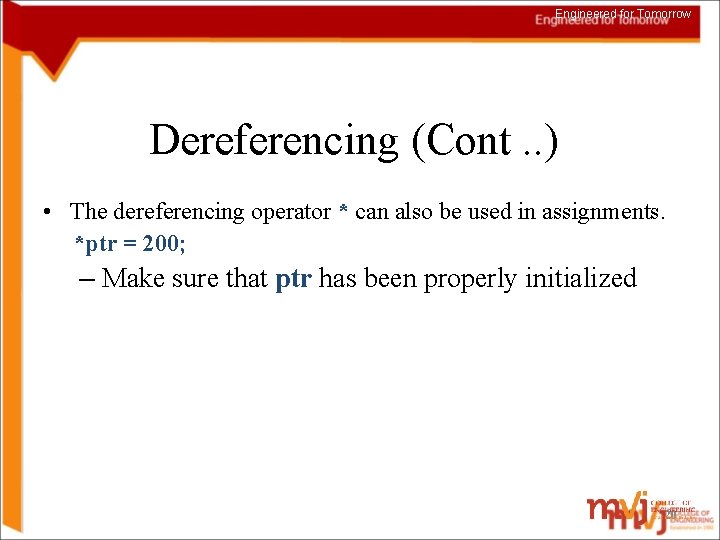
Engineered for Tomorrow Dereferencing (Cont. . ) • The dereferencing operator * can also be used in assignments. *ptr = 200; – Make sure that ptr has been properly initialized 20

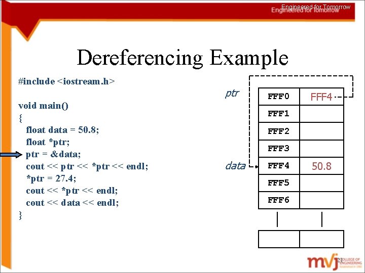
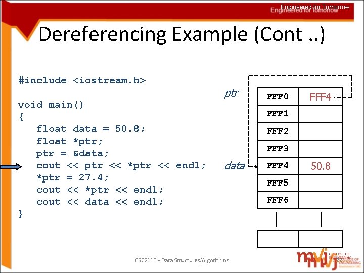
Engineered for Tomorrow Dereferencing Example #include <iostream. h> void main() { float data = 50. 8; float *ptr; ptr = &data; cout << ptr << *ptr << endl; *ptr = 27. 4; cout << *ptr << endl; cout << data << endl; } ptr FFF 0 FFF 4 FFF 1 FFF 2 FFF 3 data FFF 4 50. 8 FFF 5 FFF 6 Output: 21

Engineered for Tomorrow Dereferencing Example (Cont. . ) #include <iostream. h> void main() { float data = 50. 8; float *ptr; ptr = &data; cout << ptr << *ptr << endl; *ptr = 27. 4; cout << *ptr << endl; cout << data << endl; } ptr FFF 0 FFF 4 FFF 1 FFF 2 FFF 3 data FFF 4 50. 8 FFF 5 FFF 6 Output: FFF 4 50. 80 CSC 2110 - Data Structures/Algorithms 22

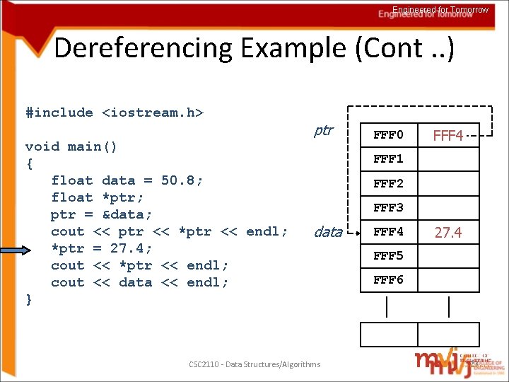
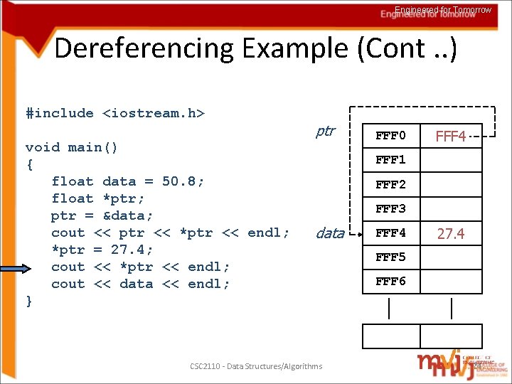
Engineered for Tomorrow Dereferencing Example (Cont. . ) #include <iostream. h> void main() { float data = 50. 8; float *ptr; ptr = &data; cout << ptr << *ptr << endl; *ptr = 27. 4; cout << *ptr << endl; cout << data << endl; } ptr FFF 0 FFF 4 FFF 1 FFF 2 FFF 3 data FFF 4 27. 4 FFF 5 FFF 6 Output: CSC 2110 - Data Structures/Algorithms 23

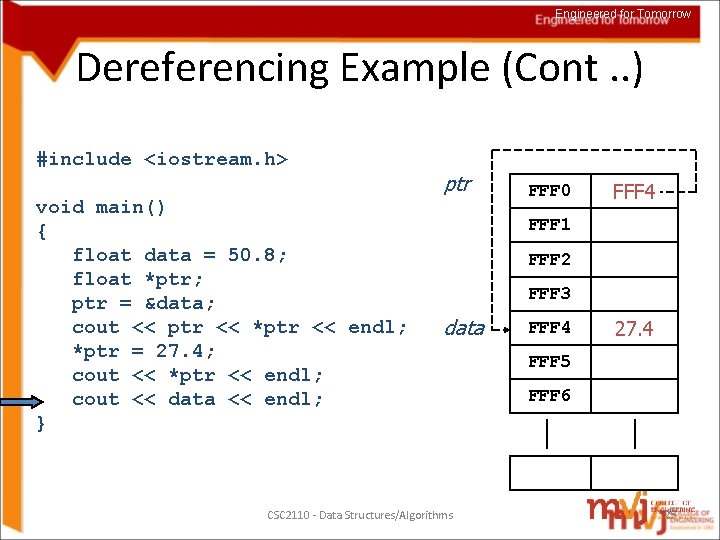
Engineered for Tomorrow Dereferencing Example (Cont. . ) #include <iostream. h> void main() { float data = 50. 8; float *ptr; ptr = &data; cout << ptr << *ptr << endl; *ptr = 27. 4; cout << *ptr << endl; cout << data << endl; } ptr FFF 0 FFF 4 FFF 1 FFF 2 FFF 3 data FFF 4 27. 4 FFF 5 FFF 6 Output: 27. 4 CSC 2110 - Data Structures/Algorithms 24

Engineered for Tomorrow Dereferencing Example (Cont. . ) #include <iostream. h> void main() { float data = 50. 8; float *ptr; ptr = &data; cout << ptr << *ptr << endl; *ptr = 27. 4; cout << *ptr << endl; cout << data << endl; } ptr FFF 0 FFF 4 FFF 1 FFF 2 FFF 3 data FFF 4 27. 4 FFF 5 FFF 6 Output: 27. 4 CSC 2110 - Data Structures/Algorithms 25

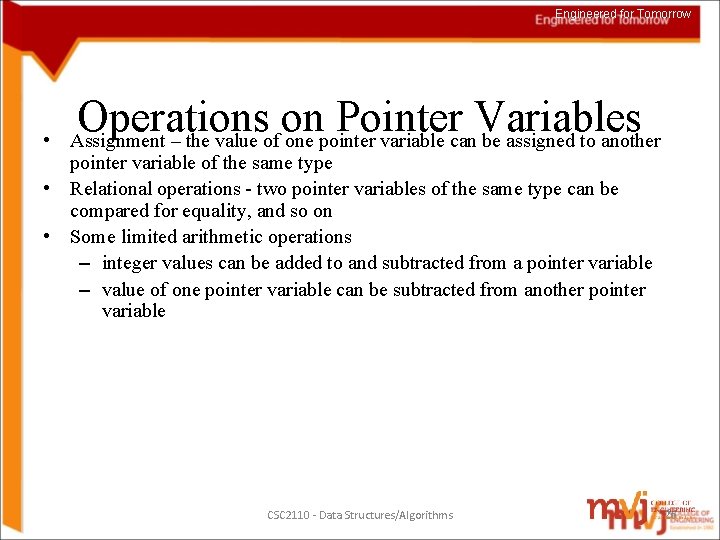
Engineered for Tomorrow • Operations on Pointer Variables Assignment – the value of one pointer variable can be assigned to another pointer variable of the same type • Relational operations - two pointer variables of the same type can be compared for equality, and so on • Some limited arithmetic operations – integer values can be added to and subtracted from a pointer variable – value of one pointer variable can be subtracted from another pointer variable CSC 2110 - Data Structures/Algorithms 26

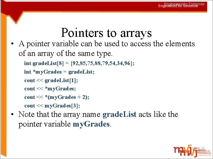
Engineered for Tomorrow Pointers to arrays • A pointer variable can be used to access the elements of an array of the same type. int grade. List[8] = {92, 85, 75, 88, 79, 54, 34, 96}; int *my. Grades = grade. List; cout << grade. List[1]; cout << *my. Grades; cout << *(my. Grades + 2); cout << my. Grades[3]; • Note that the array name grade. List acts like the pointer variable my. Grades. 27

Engineered for Tomorrow Dynamic Memory Allocation 28

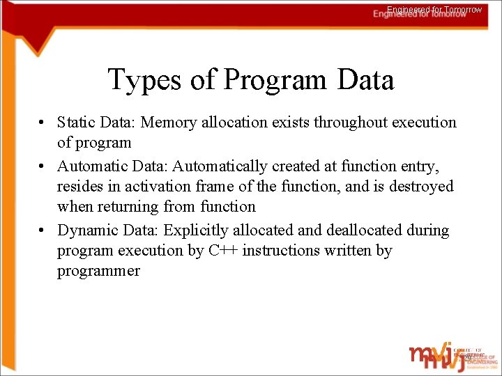
Engineered for Tomorrow Types of Program Data • Static Data: Memory allocation exists throughout execution of program • Automatic Data: Automatically created at function entry, resides in activation frame of the function, and is destroyed when returning from function • Dynamic Data: Explicitly allocated and deallocated during program execution by C++ instructions written by programmer 29

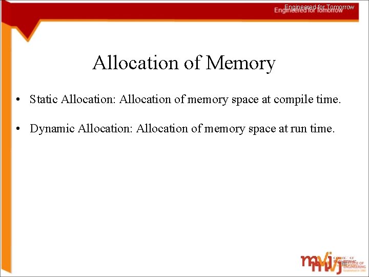
Engineered for Tomorrow Allocation of Memory • Static Allocation: Allocation of memory space at compile time. • Dynamic Allocation: Allocation of memory space at run time. 30

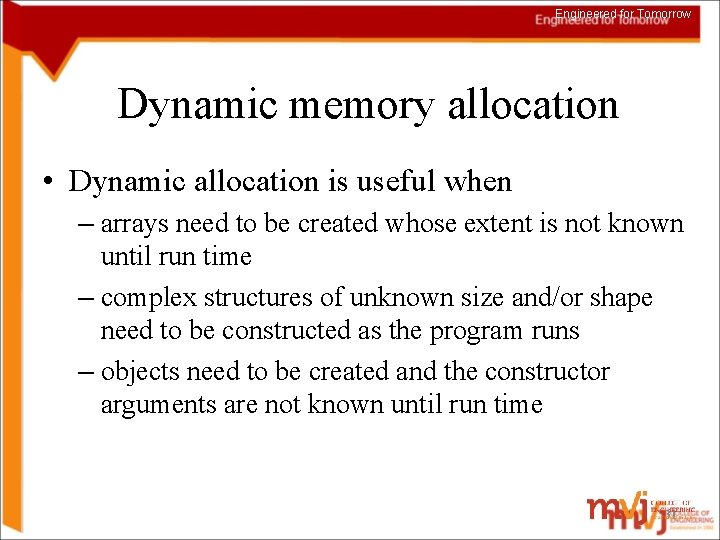
Engineered for Tomorrow Dynamic memory allocation • Dynamic allocation is useful when – arrays need to be created whose extent is not known until run time – complex structures of unknown size and/or shape need to be constructed as the program runs – objects need to be created and the constructor arguments are not known until run time 31

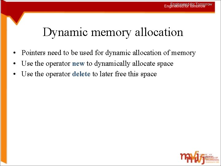
Engineered for Tomorrow Dynamic memory allocation • Pointers need to be used for dynamic allocation of memory • Use the operator new to dynamically allocate space • Use the operator delete to later free this space 32

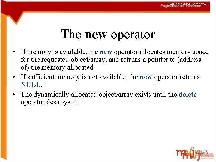
Engineered for Tomorrow The new operator • If memory is available, the new operator allocates memory space for the requested object/array, and returns a pointer to (address of) the memory allocated. • If sufficient memory is not available, the new operator returns NULL. • The dynamically allocated object/array exists until the delete operator destroys it. 33

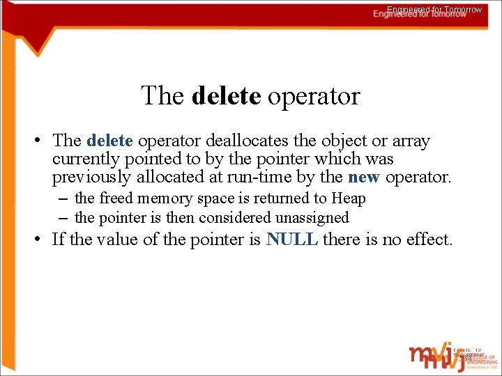
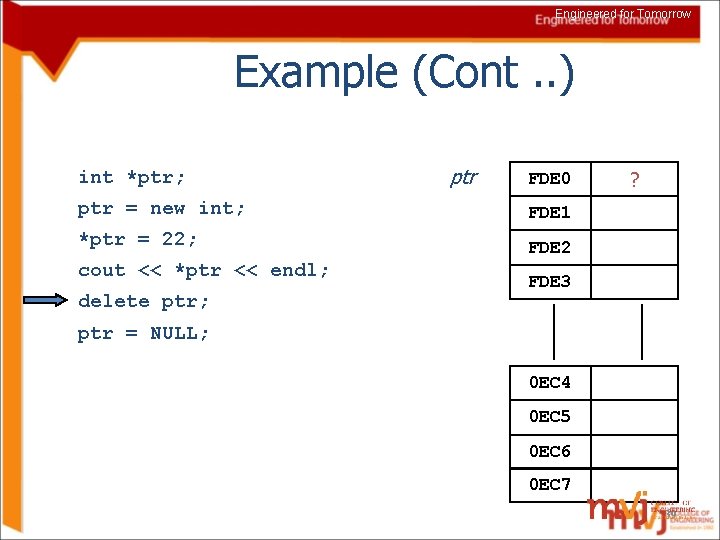
Engineered for Tomorrow The delete operator • The delete operator deallocates the object or array currently pointed to by the pointer which was previously allocated at run-time by the new operator. – the freed memory space is returned to Heap – the pointer is then considered unassigned • If the value of the pointer is NULL there is no effect. 34

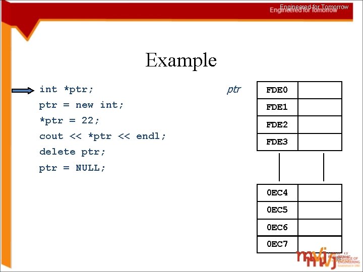
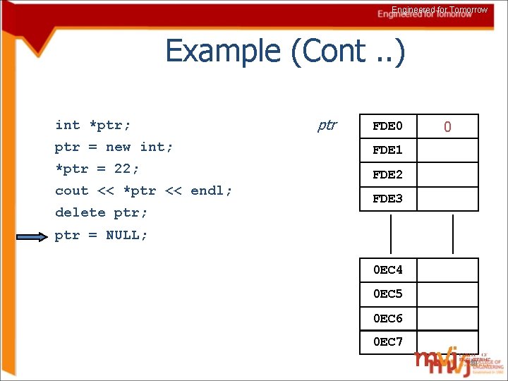
Engineered for Tomorrow Example int *ptr; ptr FDE 0 ptr = new int; FDE 1 *ptr = 22; FDE 2 cout << *ptr << endl; delete ptr; FDE 3 ptr = NULL; 0 EC 4 0 EC 5 0 EC 6 0 EC 7 35

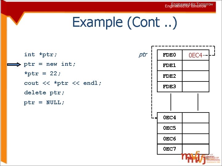
Engineered for Tomorrow Example (Cont. . ) int *ptr; ptr FDE 0 ptr = new int; FDE 1 *ptr = 22; FDE 2 cout << *ptr << endl; delete ptr; 0 EC 4 FDE 3 ptr = NULL; 0 EC 4 0 EC 5 0 EC 6 0 EC 7 36

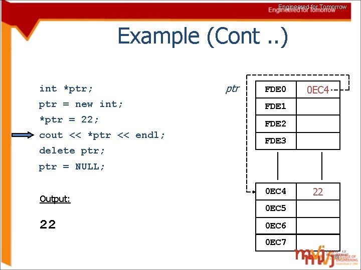
Engineered for Tomorrow Example (Cont. . ) int *ptr; ptr FDE 0 ptr = new int; FDE 1 *ptr = 22; FDE 2 cout << *ptr << endl; delete ptr; 0 EC 4 FDE 3 ptr = NULL; 0 EC 4 22 0 EC 5 0 EC 6 0 EC 7 37

Engineered for Tomorrow Example (Cont. . ) int *ptr; ptr FDE 0 ptr = new int; FDE 1 *ptr = 22; FDE 2 cout << *ptr << endl; delete ptr; 0 EC 4 FDE 3 ptr = NULL; Output: 22 0 EC 4 22 0 EC 5 0 EC 6 0 EC 7 38

Engineered for Tomorrow Example (Cont. . ) int *ptr; ptr FDE 0 ptr = new int; FDE 1 *ptr = 22; FDE 2 cout << *ptr << endl; delete ptr; ? FDE 3 ptr = NULL; 0 EC 4 0 EC 5 0 EC 6 0 EC 7 39

Engineered for Tomorrow Example (Cont. . ) int *ptr; ptr FDE 0 ptr = new int; FDE 1 *ptr = 22; FDE 2 cout << *ptr << endl; delete ptr; 0 FDE 3 ptr = NULL; 0 EC 4 0 EC 5 0 EC 6 0 EC 7 40

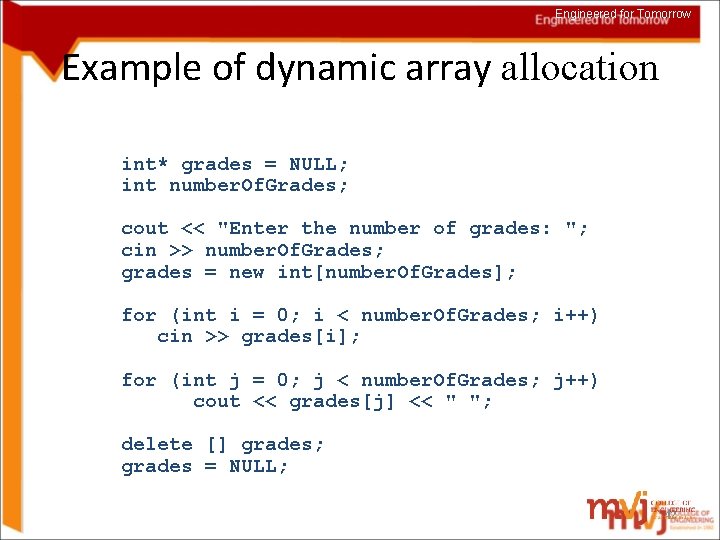
Engineered for Tomorrow Dynamic allocation and deallocation of arrays • Use the [Int. Exp] on the new statement to create an array of objects instead of a single instance. • On the delete statement use [] to indicate that an array of objects is to be deallocated. 41

Engineered for Tomorrow Example of dynamic array allocation int* grades = NULL; int number. Of. Grades; cout << "Enter the number of grades: "; cin >> number. Of. Grades; grades = new int[number. Of. Grades]; for (int i = 0; i < number. Of. Grades; i++) cin >> grades[i]; for (int j = 0; j < number. Of. Grades; j++) cout << grades[j] << " "; delete [] grades; grades = NULL; 42

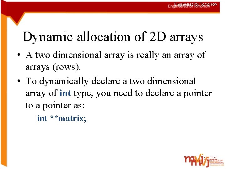
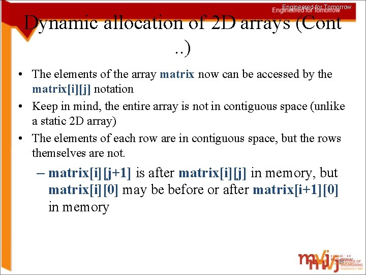
Engineered for Tomorrow Dynamic allocation of 2 D arrays • A two dimensional array is really an array of arrays (rows). • To dynamically declare a two dimensional array of int type, you need to declare a pointer to a pointer as: int **matrix; 43

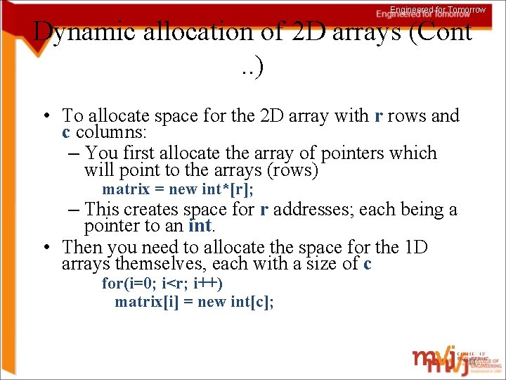
Engineered for Tomorrow Dynamic allocation of 2 D arrays (Cont. . ) • To allocate space for the 2 D array with r rows and c columns: – You first allocate the array of pointers which will point to the arrays (rows) matrix = new int*[r]; – This creates space for r addresses; each being a pointer to an int. • Then you need to allocate the space for the 1 D arrays themselves, each with a size of c for(i=0; i<r; i++) matrix[i] = new int[c]; 44

Engineered for Tomorrow Dynamic allocation of 2 D arrays (Cont. . ) • The elements of the array matrix now can be accessed by the matrix[i][j] notation • Keep in mind, the entire array is not in contiguous space (unlike a static 2 D array) • The elements of each row are in contiguous space, but the rows themselves are not. – matrix[i][j+1] is after matrix[i][j] in memory, but matrix[i][0] may be before or after matrix[i+1][0] in memory 45

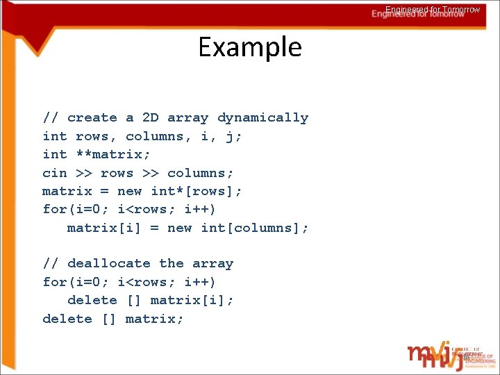
Engineered for Tomorrow Example // create a 2 D array dynamically int rows, columns, i, j; int **matrix; cin >> rows >> columns; matrix = new int*[rows]; for(i=0; i<rows; i++) matrix[i] = new int[columns]; // deallocate the array for(i=0; i<rows; i++) delete [] matrix[i]; delete [] matrix; 46

Engineered for Tomorrow Passing pointers to a function 47

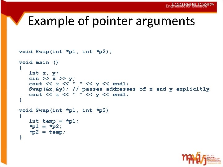
Engineered for Tomorrow Pointers as arguments to functions • Pointers can be passed to functions just like other types. • Just as with any other argument, verify that the number and type of arguments in function invocation match the prototype (and function header). 48

Engineered for Tomorrow Example of pointer arguments void Swap(int *p 1, int *p 2); void main () { int x, y; cin >> x >> y; cout << x << " " << y << endl; Swap(&x, &y); // passes addresses of x and y explicitly cout << x << " " << y << endl; } void Swap(int *p 1, int *p 2) { int temp = *p 1; *p 1 = *p 2; *p 2 = temp; } 49

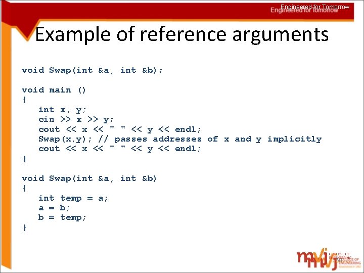
Engineered for Tomorrow Example of reference arguments void Swap(int &a, int &b); void main () { int x, y; cin >> x >> y; cout << x << " " << y << endl; Swap(x, y); // passes addresses of x and y implicitly cout << x << " " << y << endl; } void Swap(int &a, int &b) { int temp = a; a = b; b = temp; } 50

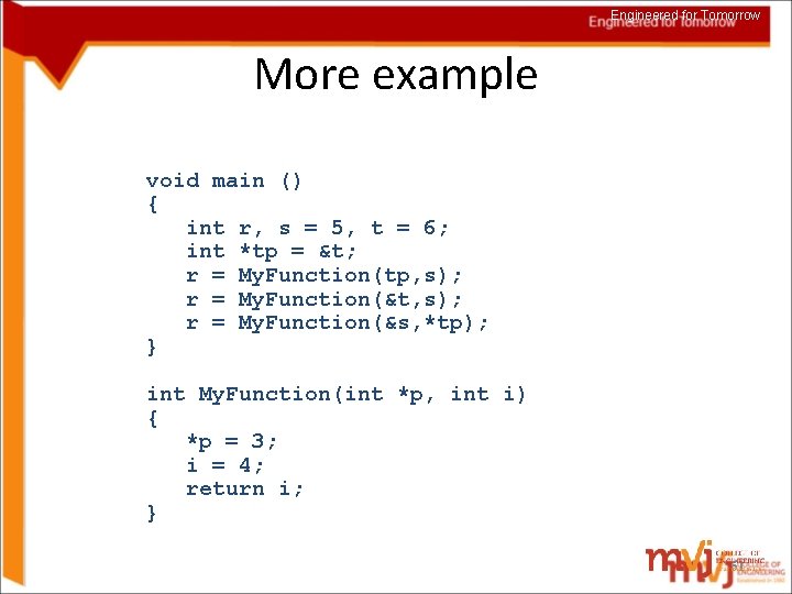
Engineered for Tomorrow More example void main () { int r, s = 5, t = 6; int *tp = &t; r = My. Function(tp, s); r = My. Function(&t, s); r = My. Function(&s, *tp); } int My. Function(int *p, int i) { *p = 3; i = 4; return i; } 51

Engineered for Tomorrow Memory leaks and Dangling Pointers 52

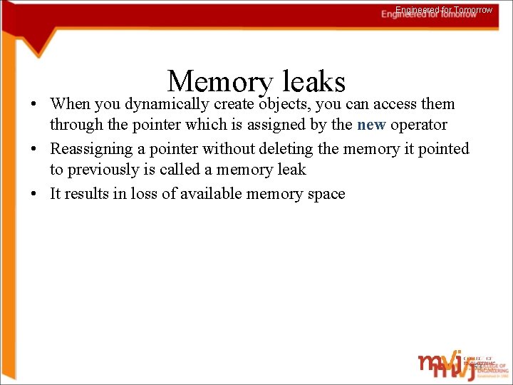
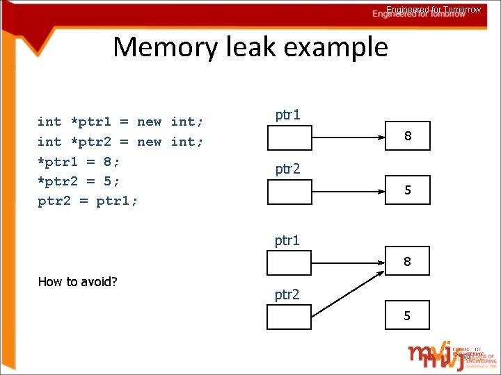
Engineered for Tomorrow Memory leaks • When you dynamically create objects, you can access them through the pointer which is assigned by the new operator • Reassigning a pointer without deleting the memory it pointed to previously is called a memory leak • It results in loss of available memory space 53

Engineered for Tomorrow Memory leak example int *ptr 1 = new int; int *ptr 2 = new int; *ptr 1 = 8; *ptr 2 = 5; ptr 2 = ptr 1; ptr 1 8 ptr 2 5 ptr 1 8 How to avoid? ptr 2 5 54

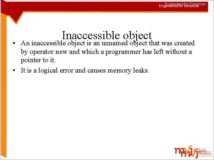
Engineered for Tomorrow Inaccessible object • An inaccessible object is an unnamed object that was created by operator new and which a programmer has left without a pointer to it. • It is a logical error and causes memory leaks. 55

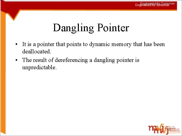
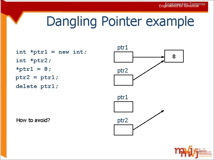
Engineered for Tomorrow Dangling Pointer • It is a pointer that points to dynamic memory that has been deallocated. • The result of dereferencing a dangling pointer is unpredictable. 56

Engineered for Tomorrow Dangling Pointer example int *ptr 1 = new int; int *ptr 2; *ptr 1 = 8; ptr 2 = ptr 1; delete ptr 1; ptr 1 8 ptr 2 ptr 1 How to avoid? ptr 2 57

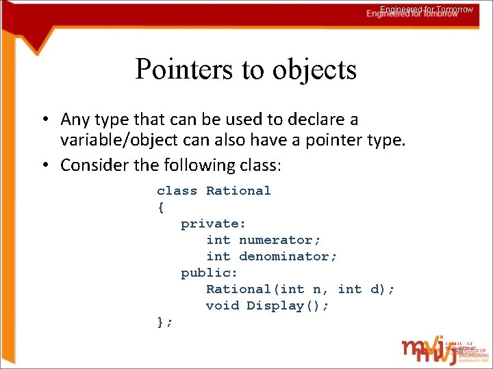
Engineered for Tomorrow Pointers to objects • Any type that can be used to declare a variable/object can also have a pointer type. • Consider the following class: class Rational { private: int numerator; int denominator; public: Rational(int n, int d); void Display(); }; 58

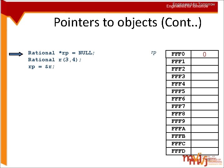
Engineered for Tomorrow Pointers to objects (Cont. . ) Rational *rp = NULL; Rational r(3, 4); rp = &r; rp FFF 0 FFF 1 FFF 2 FFF 3 FFF 4 FFF 5 FFF 6 FFF 7 FFF 8 FFF 9 FFFA FFFB FFFC FFFD 0 59

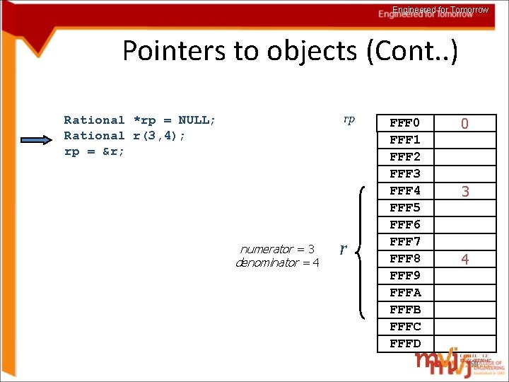
Engineered for Tomorrow Pointers to objects (Cont. . ) rp Rational *rp = NULL; Rational r(3, 4); rp = &r; numerator = 3 denominator = 4 r FFF 0 FFF 1 FFF 2 FFF 3 FFF 4 FFF 5 FFF 6 FFF 7 FFF 8 FFF 9 FFFA FFFB FFFC FFFD 0 3 4 60

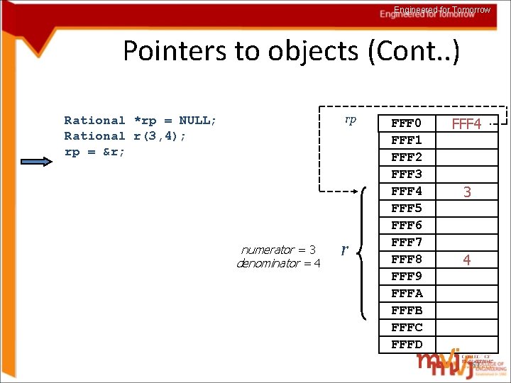
Engineered for Tomorrow Pointers to objects (Cont. . ) rp Rational *rp = NULL; Rational r(3, 4); rp = &r; numerator = 3 denominator = 4 r FFF 0 FFF 1 FFF 2 FFF 3 FFF 4 FFF 5 FFF 6 FFF 7 FFF 8 FFF 9 FFFA FFFB FFFC FFFD FFF 4 3 4 61

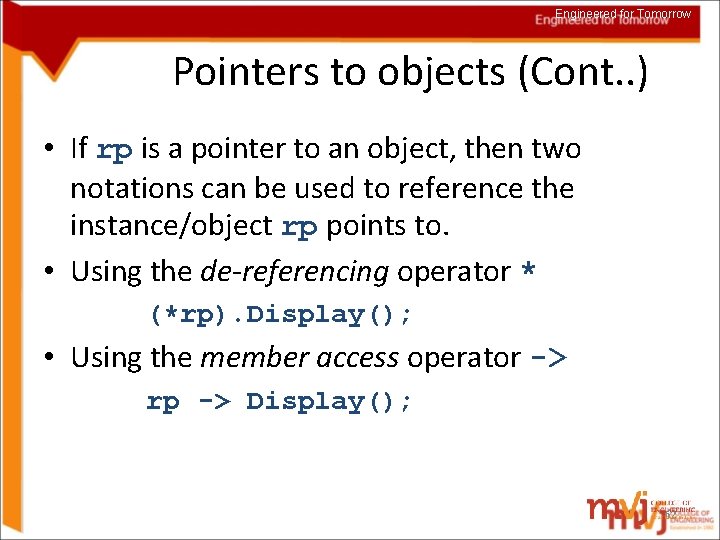
Engineered for Tomorrow Pointers to objects (Cont. . ) • If rp is a pointer to an object, then two notations can be used to reference the instance/object rp points to. • Using the de-referencing operator * (*rp). Display(); • Using the member access operator -> rp -> Display(); 62

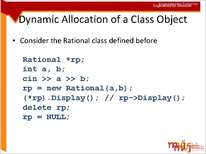
Engineered for Tomorrow Dynamic Allocation of a Class Object • Consider the Rational class defined before Rational *rp; int a, b; cin >> a >> b; rp = new Rational(a, b); (*rp). Display(); // rp->Display(); delete rp; rp = NULL; 63

Analysis of Algorithms • Efficiency: – Running time – Space used • Efficiency as a function of input size: – Number of data elements (numbers, points) – A number of bits in an input number

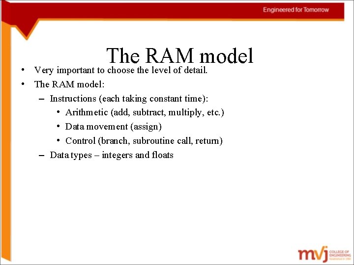
The RAM model Very important to choose the level of detail. • • The RAM model: – Instructions (each taking constant time): • Arithmetic (add, subtract, multiply, etc. ) • Data movement (assign) • Control (branch, subroutine call, return) – Data types – integers and floats

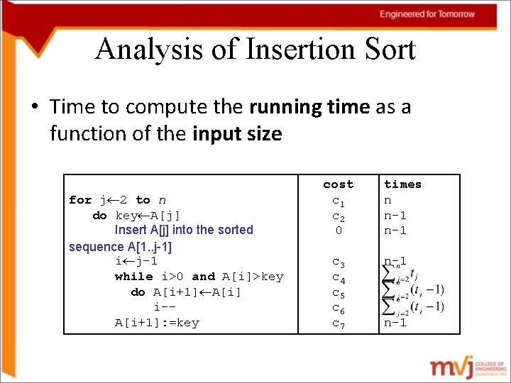
Analysis of Insertion Sort • Time to compute the running time as a function of the input size for j¬ 2 to n do key¬A[j] Insert A[j] into the sorted sequence A[1. . j-1] i¬j-1 while i>0 and A[i]>key do A[i+1]¬A[i] i-A[i+1]: =key cost c 1 c 2 0 c 3 c 4 c 5 c 6 c 7 times n n-1 n-1

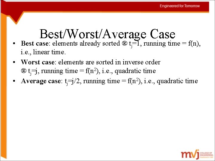
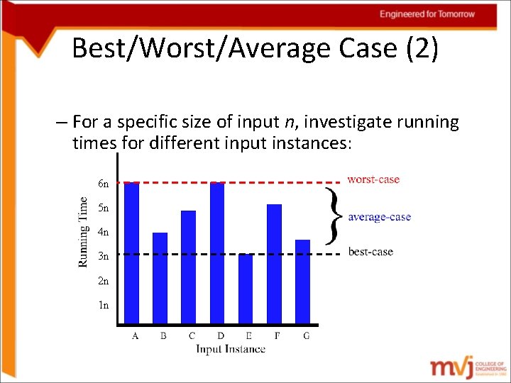
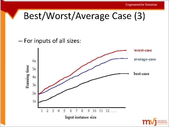
Best/Worst/Average Case • Best case: elements already sorted ® tj=1, running time = f(n), i. e. , linear time. • Worst case: elements are sorted in inverse order ® tj=j, running time = f(n 2), i. e. , quadratic time • Average case: tj=j/2, running time = f(n 2), i. e. , quadratic time

Best/Worst/Average Case (2) – For a specific size of input n, investigate running times for different input instances: 6 n 5 n 4 n 3 n 2 n 1 n

Best/Worst/Average Case (3) – For inputs of all sizes: worst-case average-case Running time 6 n 5 n best-case 4 n 3 n 2 n 1 n 1 2 3 4 5 6 7 8 9 10 11 12 …. . Input instance size

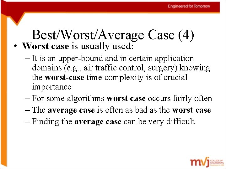
Best/Worst/Average Case (4) • Worst case is usually used: – It is an upper-bound and in certain application domains (e. g. , air traffic control, surgery) knowing the worst-case time complexity is of crucial importance – For some algorithms worst case occurs fairly often – The average case is often as bad as the worst case – Finding the average case can be very difficult

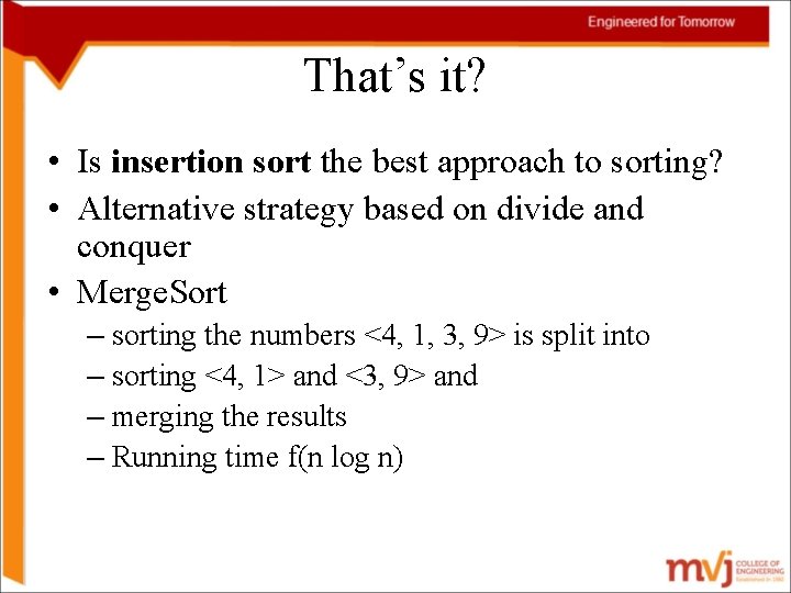
That’s it? • Is insertion sort the best approach to sorting? • Alternative strategy based on divide and conquer • Merge. Sort – sorting the numbers <4, 1, 3, 9> is split into – sorting <4, 1> and <3, 9> and – merging the results – Running time f(n log n)

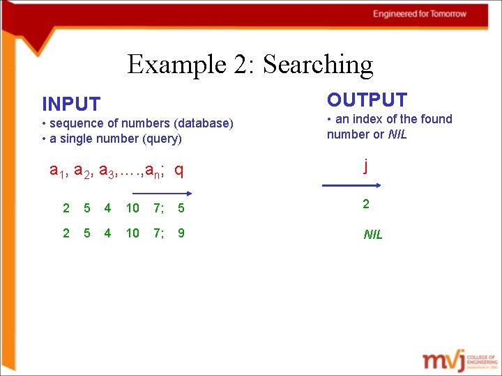
Example 2: Searching OUTPUT INPUT • sequence of numbers (database) • a single number (query) a 1, a 2, a 3, …. , an; q • an index of the found number or NIL j 2 5 4 10 7; 5 2 2 5 4 10 7; 9 NIL

Searching (2) INPUT: A[1. . n] – an array of integers, q – an integer. OUTPUT: an index j such that A[j] = q. NIL, if "j (1£j£n): A[j] ¹ q j¬ 1 while j £ n and A[j] ¹ q do j++ if j £ n then return j else return NIL n n Worst-case running time: f(n), average-case: f(n/2) We can’t do better. This is a lower bound for the problem of searching in an arbitrary sequence.

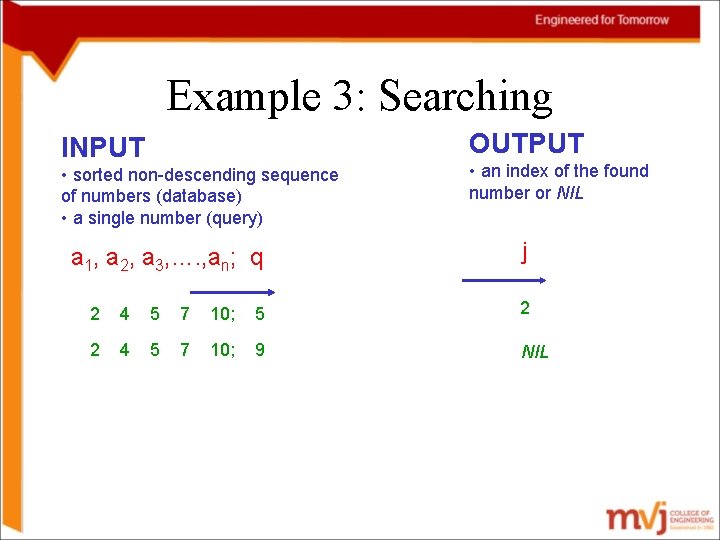
Example 3: Searching OUTPUT INPUT • sorted non-descending sequence of numbers (database) • a single number (query) a 1, a 2, a 3, …. , an; q • an index of the found number or NIL j 2 4 5 7 10; 5 2 2 4 5 7 10; 9 NIL

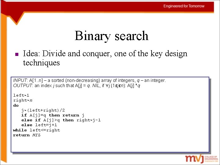
Binary search n Idea: Divide and conquer, one of the key design techniques INPUT: A[1. . n] – a sorted (non-decreasing) array of integers, q – an integer. OUTPUT: an index j such that A[j] = q. NIL, if "j (1£j£n): A[j] ¹ q left¬ 1 right¬n do j¬(left+right)/2 if A[j]=q then return j else if A[j]>q then right¬j-1 else left=j+1 while left<=right return NIL

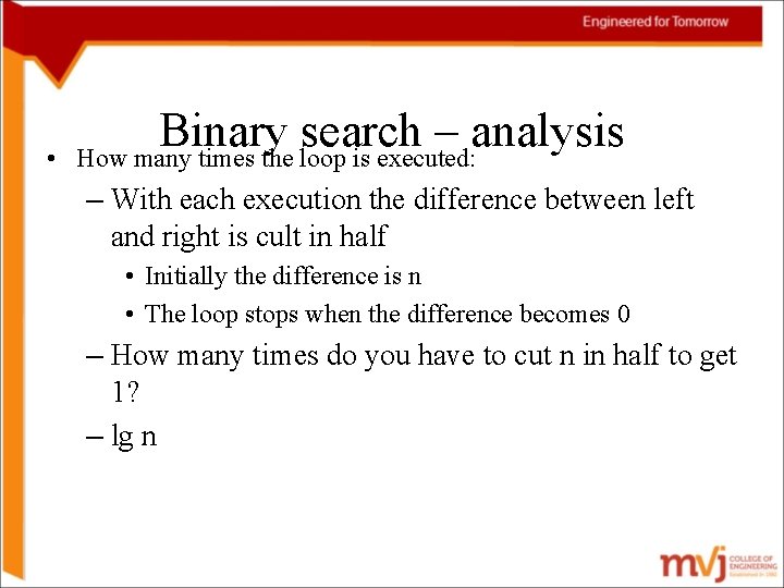
• Binary search – analysis How many times the loop is executed: – With each execution the difference between left and right is cult in half • Initially the difference is n • The loop stops when the difference becomes 0 – How many times do you have to cut n in half to get 1? – lg n

The Goals of this Course • The main things that we will try to learn in this course: – To be able to think “algorithmically”, to get the spirit of how algorithms are designed – To get to know a toolbox of classical algorithms – To learn a number of algorithm design techniques (such as divide-and-conquer) – To learn reason (in a formal way) about the efficiency and the correctness of algorithms

The Concept of Abstraction • An abstraction is a view or representation of an entity that includes only the most significant attributes • The concept of abstraction is fundamental in programming (and computer science) • Nearly all programming languages support process abstraction with subprograms • Nearly all programming languages designed since 1980 support data abstraction 1 -78

Introduction to Data Abstraction • An abstract data type is a user-defined data type that satisfies the following two conditions: – The representation of, and operations on, objects of the type are defined in a single syntactic unit – The representation of objects of the type is hidden from the program units that use these objects, so the only operations possible are those provided in the type's definition 1 -79

Advantages of Data Abstraction • Advantage of the first condition – Program organization, modifiability (everything associated with a data structure is together), and separate compilation • Advantage the secondition – Reliability--by hiding the data representations, user code cannot directly access objects of the type or depend on the representation, allowing the representation to be changed without affecting user code 1 -80

Language Requirements for ADTs • A syntactic unit in which to encapsulate the type definition • A method of making type names and subprogram headers visible to clients, while hiding actual definitions • Some primitive operations must be built into the language processor 1 -81

Classification of ADT operations • Creator (constructor) – Group. Users(String user. IDs[ ]) • Producer – add. User(String user. ID) • Mutator – set. User. Email(String email) • Observer – is. Member (String user. ID)

Algorithm Specification • 1. 2. 1 Introduction – An algorithm is a finite set of instructions that accomplishes a particular task. – Criteria • input: zero or more quantities that are externally supplied • output: at least one quantity is produced • definiteness: clear and unambiguous • finiteness: terminate after a finite number of steps • effectiveness: instruction is basic enough to be carried out – A program does not have to satisfy the finiteness criteria.

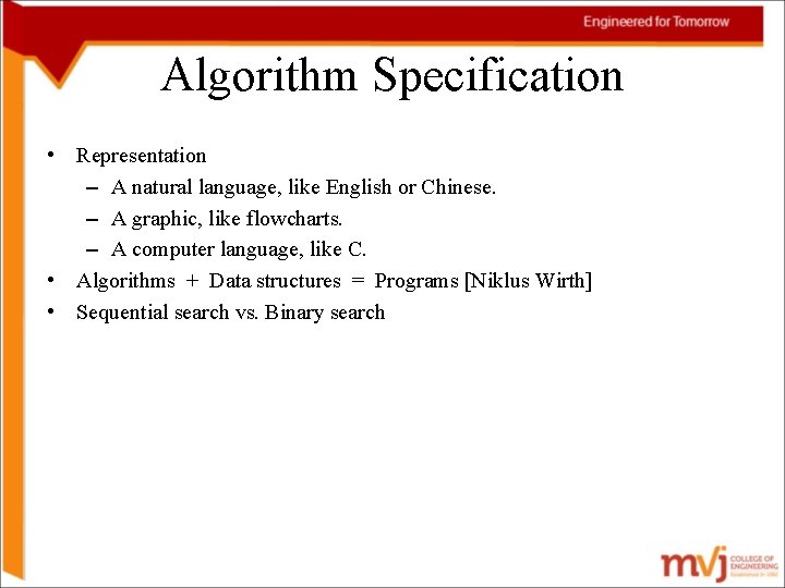
Algorithm Specification • Representation – A natural language, like English or Chinese. – A graphic, like flowcharts. – A computer language, like C. • Algorithms + Data structures = Programs [Niklus Wirth] • Sequential search vs. Binary search

Algorithm Specification • Example 1. 1 [Selection sort]: – From those integers that are currently unsorted, find the smallest and place it next in the sorted list. i [0] [1] [2] [3] [4] 0 1 2 3 30 10 10 10 30 20 20 20 50 50 40 30 30 40 40 50 40 40 20 20 30 50 50

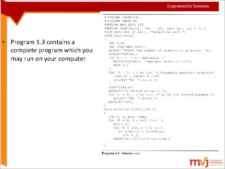
• Program 1. 3 contains a complete program which you may run on your computer

Algorithm Specification • • Example 1. 2 [Binary search]: [0] [1] [2] [3] [4] 8 14 26 30 43 left right middle list[middle] : searchnum 0 6 3 30 < 43 4 6 5 50 > 43 4 43 == 43 0 6 3 30 > 18 0 2 1 14 < 18 2 26 > 18 2 1 Searching a sorted list while (there are more integers to check) { middle = (left + right) / 2; if (searchnum < list[middle]) right = middle - 1; else if (searchnum == list[middle]) return middle; else left = middle + 1; } [5] 50 [6] 52

int binsearch(int list[], int searchnum, int left, int right) { /* search list[0] <= list[1] <= … <= list[n-1] for searchnum. Return its position if found. Otherwise return -1 */ int middle; while (left <= right) { middle = (left + right)/2; switch (COMPARE(list[middle], searchnum)) { case -1: left = middle + 1; break; case 0 : return middle; case 1 : right = middle – 1; } } return -1; }

Algorithm Specification • Recursive algorithms – Beginning programmer view a function as something that is invoked (called) by another function • It executes its code and then returns control to the calling function.

Algorithm Specification – This perspective ignores the fact that functions can call themselves (direct recursion). – They may call other functions that invoke the calling function again (indirect recursion). • extremely powerful • frequently allow us to express an otherwise complex process in very clear term – We should express a recursive algorithm when the problem itself is defined recursively.

Algorithm Specification • Example 1. 3 [Binary search]:

• Example 1. 4 [Permutations]: lv 0 perm: i=0, lv 0 SWAP: i=0, lv 1 perm: i=1, lv 1 SWAP: i=1, lv 2 perm: i=2, print: abc lv 1 SWAP: i=1, lv 2 perm: i=2, print: acb lv 1 SWAP: i=1, lv 0 SWAP: i=0, lv 1 perm: i=1, lv 1 SWAP: i=1, lv 2 perm: i=2, print: bac lv 1 SWAP: i=1, lv 2 perm: i=2, print: bca lv 1 SWAP: i=1, lv 0 SWAP: i=0, lv 1 perm: i=1, lv 1 SWAP: i=1, lv 2 perm: i=2, print: cba lv 1 SWAP: i=1, lv 2 perm: i=2, print: cab lv 1 SWAP: i=1, lv 0 SWAP: i=0, n=2 j=0 n=2 j=1 n=2 abc abc abc j=1 abc j=2 abc n=2 acb j=2 j=0 j=1 n=2 acb abc bac bac j=1 bac j=2 bac n=2 bca j=2 j=1 j=2 n=2 j=1 n=2 bca bac abc cba cba j=1 cba j=2 cba n=2 cab j=2 cba

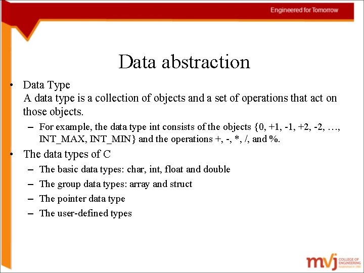
Data abstraction • Data Type A data type is a collection of objects and a set of operations that act on those objects. – For example, the data type int consists of the objects {0, +1, -1, +2, -2, …, INT_MAX, INT_MIN} and the operations +, -, *, /, and %. • The data types of C – – The basic data types: char, int, float and double The group data types: array and struct The pointer data type The user-defined types

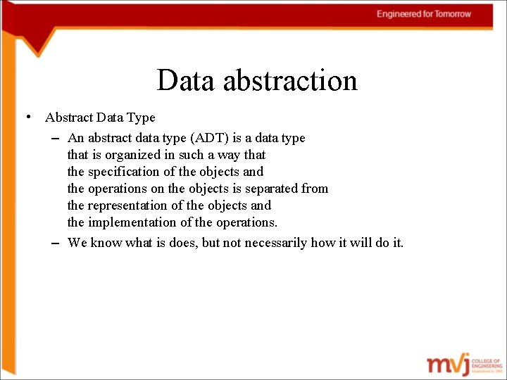
Data abstraction • Abstract Data Type – An abstract data type (ADT) is a data type that is organized in such a way that the specification of the objects and the operations on the objects is separated from the representation of the objects and the implementation of the operations. – We know what is does, but not necessarily how it will do it.

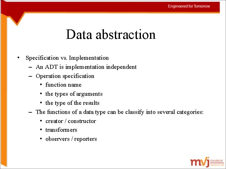
Data abstraction • Specification vs. Implementation – An ADT is implementation independent – Operation specification • function name • the types of arguments • the type of the results – The functions of a data type can be classify into several categories: • creator / constructor • transformers • observers / reporters

Data abstraction • Example 1. 5 [Abstract data type Natural_Number] : : = is defined as

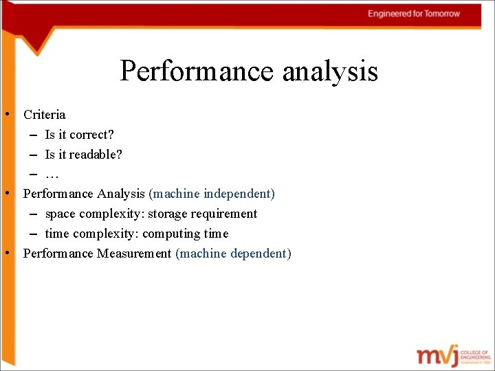
Performance analysis • Criteria – Is it correct? – Is it readable? – … • Performance Analysis (machine independent) – space complexity: storage requirement – time complexity: computing time • Performance Measurement (machine dependent)

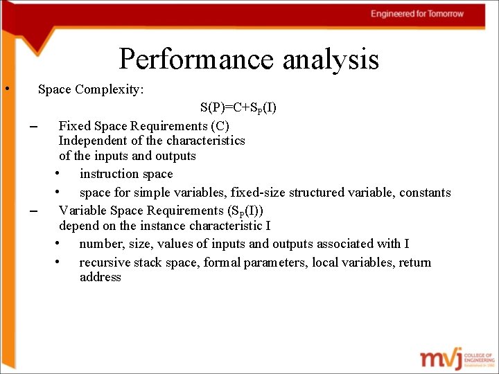
Performance analysis • Space Complexity: – – S(P)=C+SP(I) Fixed Space Requirements (C) Independent of the characteristics of the inputs and outputs • instruction space • space for simple variables, fixed-size structured variable, constants Variable Space Requirements (SP(I)) depend on the instance characteristic I • number, size, values of inputs and outputs associated with I • recursive stack space, formal parameters, local variables, return address

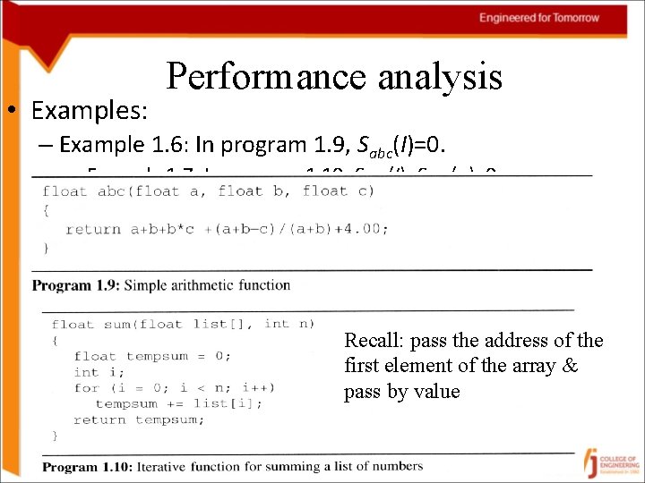
• Examples: Performance analysis – Example 1. 6: In program 1. 9, Sabc(I)=0. • Example 1. 7: In program 1. 10, Ssum(I)=Ssum(n)=0. Recall: pass the address of the first element of the array & pass by value

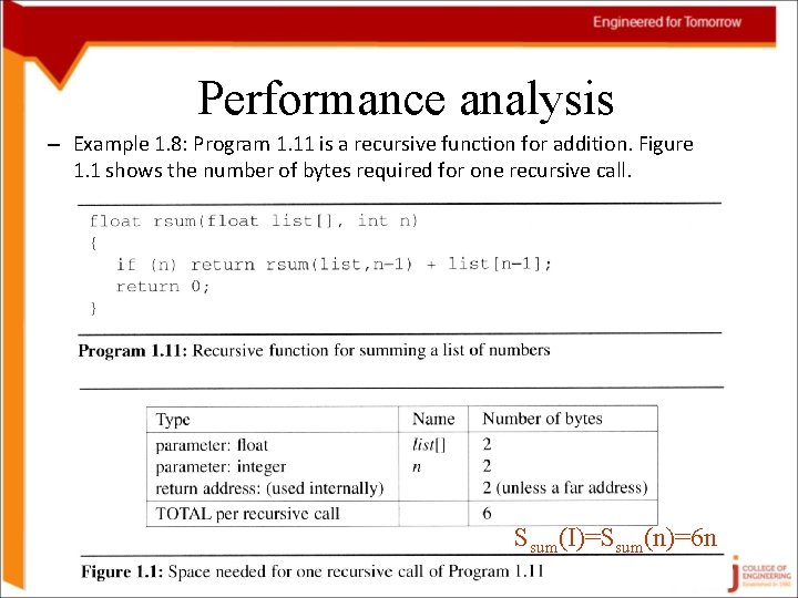
Performance analysis – Example 1. 8: Program 1. 11 is a recursive function for addition. Figure 1. 1 shows the number of bytes required for one recursive call. Ssum(I)=Ssum(n)=6 n

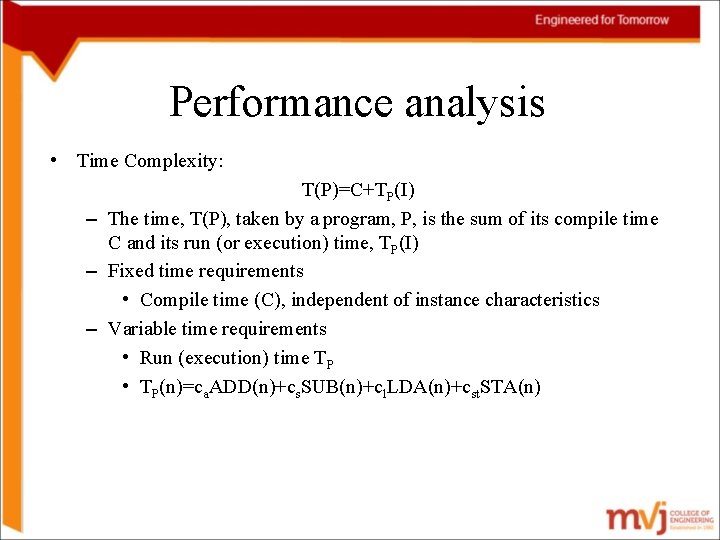
Performance analysis • Time Complexity: T(P)=C+TP(I) – The time, T(P), taken by a program, P, is the sum of its compile time C and its run (or execution) time, TP(I) – Fixed time requirements • Compile time (C), independent of instance characteristics – Variable time requirements • Run (execution) time TP • TP(n)=ca. ADD(n)+cs. SUB(n)+cl. LDA(n)+cst. STA(n)

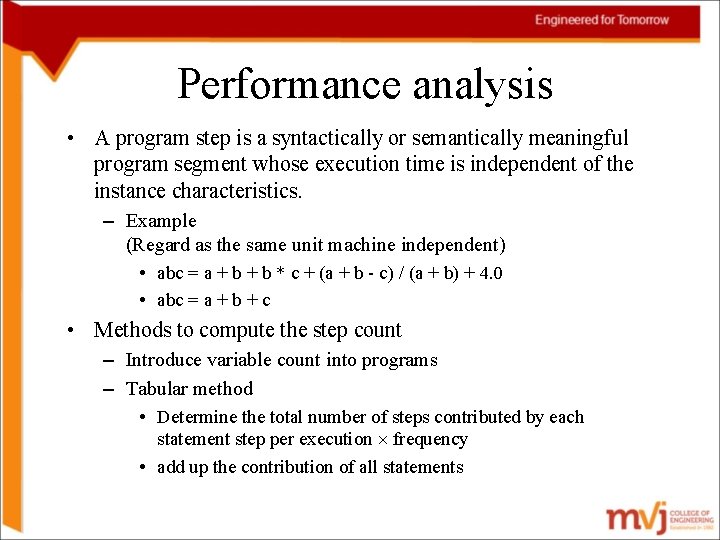
Performance analysis • A program step is a syntactically or semantically meaningful program segment whose execution time is independent of the instance characteristics. – Example (Regard as the same unit machine independent) • abc = a + b * c + (a + b - c) / (a + b) + 4. 0 • abc = a + b + c • Methods to compute the step count – Introduce variable count into programs – Tabular method • Determine the total number of steps contributed by each statement step per execution frequency • add up the contribution of all statements

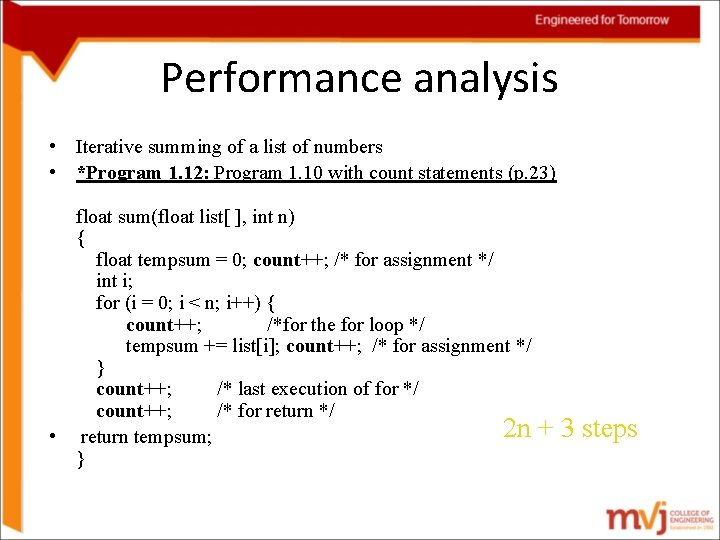
Performance analysis • Iterative summing of a list of numbers • *Program 1. 12: Program 1. 10 with count statements (p. 23) float sum(float list[ ], int n) { float tempsum = 0; count++; /* for assignment */ int i; for (i = 0; i < n; i++) { count++; /*for the for loop */ tempsum += list[i]; count++; /* for assignment */ } count++; /* last execution of for */ count++; /* for return */ 2 n • return tempsum; } + 3 steps

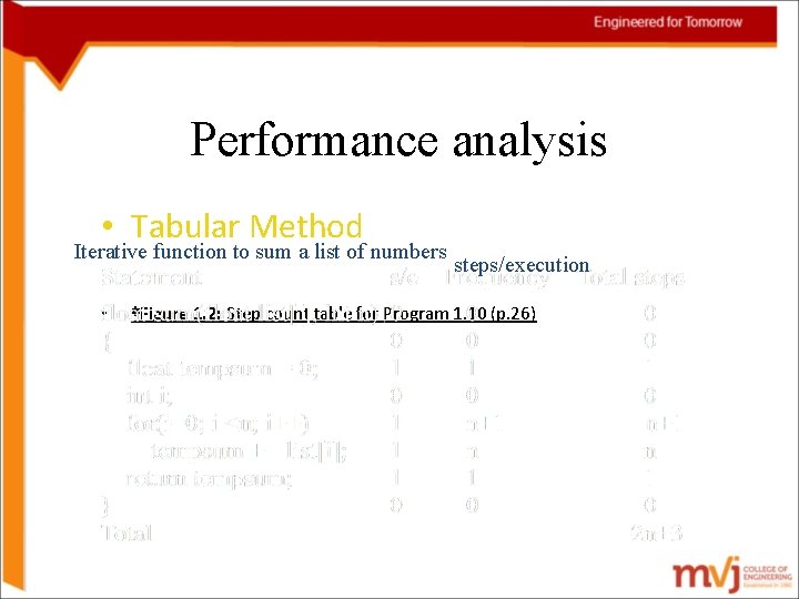
Performance analysis • Tabular Method Iterative function to sum a list of numbers • steps/execution *Figure 1. 2: Step count table for Program 1. 10 (p. 26)

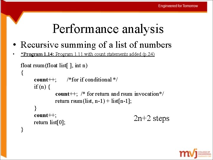
Performance analysis • Recursive summing of a list of numbers • *Program 1. 14: Program 1. 11 with count statements added (p. 24) float rsum(float list[ ], int n) { count++; /*for if conditional */ if (n) { count++; /* for return and rsum invocation*/ return rsum(list, n-1) + list[n-1]; } count++; 2 n+2 steps return list[0]; }

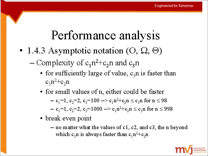
Performance analysis • 1. 4. 3 Asymptotic notation (O, , ) – Complexity of c 1 n 2+c 2 n and c 3 n • for sufficiently large of value, c 3 n is faster than c 1 n 2+c 2 n • for small values of n, either could be faster – c 1=1, c 2=2, c 3=100 --> c 1 n 2+c 2 n c 3 n for n 98 – c 1=1, c 2=2, c 3=1000 --> c 1 n 2+c 2 n c 3 n for n 998 • break even point – no matter what the values of c 1, c 2, and c 3, the n beyond which c 3 n is always faster than c 1 n 2+c 2 n

Performance analysis • Definition: [Big “oh’’] – f(n) = O(g(n)) iff there exist positive constants c and n 0 such that f(n) cg(n) for all n, n n 0. • Definition: [Omega] – f(n) = (g(n)) (read as “f of n is omega of g of n”) iff there exist positive constants c and n 0 such that f(n) cg(n) for all n, n n 0. • Definition: [Theta] – f(n) = (g(n)) (read as “f of n is theta of g of n”) iff there exist positive constants c 1, c 2, and n 0 such that c 1 g(n) f(n) c 2 g(n) for all n, n n 0.

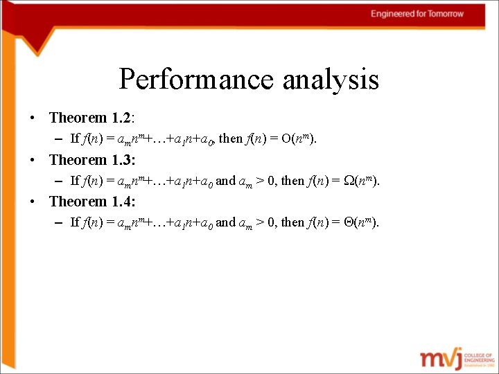
Performance analysis • Theorem 1. 2: – If f(n) = amnm+…+a 1 n+a 0, then f(n) = O(nm). • Theorem 1. 3: – If f(n) = amnm+…+a 1 n+a 0 and am > 0, then f(n) = (nm). • Theorem 1. 4: – If f(n) = amnm+…+a 1 n+a 0 and am > 0, then f(n) = (nm).

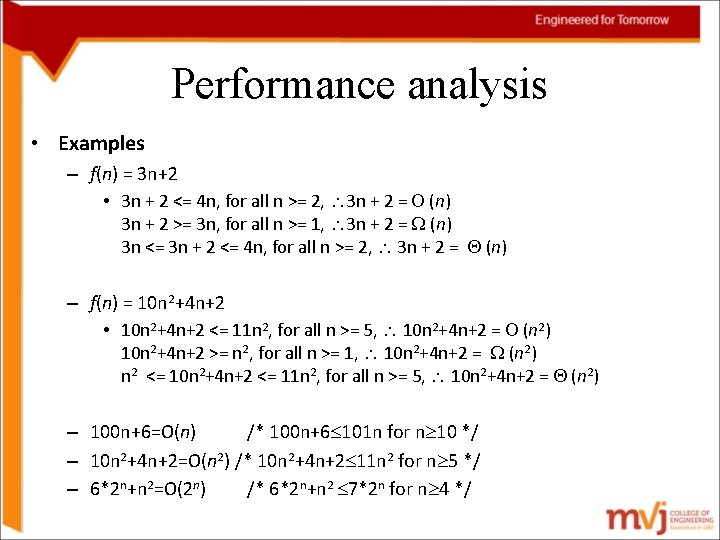
Performance analysis • Examples – f(n) = 3 n+2 • 3 n + 2 <= 4 n, for all n >= 2, 3 n + 2 = (n) 3 n + 2 >= 3 n, for all n >= 1, 3 n + 2 = (n) 3 n <= 3 n + 2 <= 4 n, for all n >= 2, 3 n + 2 = (n) – f(n) = 10 n 2+4 n+2 • 10 n 2+4 n+2 <= 11 n 2, for all n >= 5, 10 n 2+4 n+2 = (n 2) 10 n 2+4 n+2 >= n 2, for all n >= 1, 10 n 2+4 n+2 = (n 2) n 2 <= 10 n 2+4 n+2 <= 11 n 2, for all n >= 5, 10 n 2+4 n+2 = (n 2) – 100 n+6=O(n) /* 100 n+6 101 n for n 10 */ – 10 n 2+4 n+2=O(n 2) /* 10 n 2+4 n+2 11 n 2 for n 5 */ – 6*2 n+n 2=O(2 n) /* 6*2 n+n 2 7*2 n for n 4 */

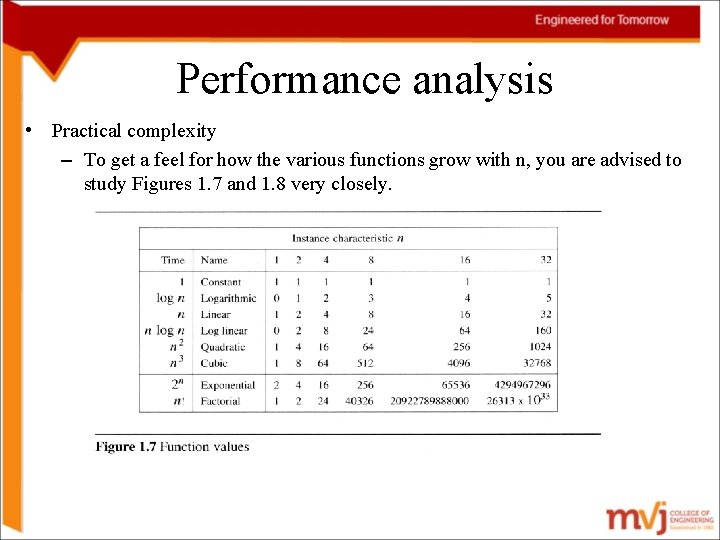
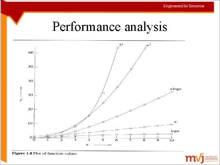
Performance analysis • Practical complexity – To get a feel for how the various functions grow with n, you are advised to study Figures 1. 7 and 1. 8 very closely.

Performance analysis

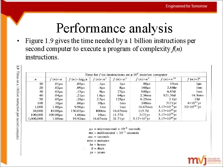
Performance analysis • Figure 1. 9 gives the time needed by a 1 billion instructions per second computer to execute a program of complexity f(n) instructions.

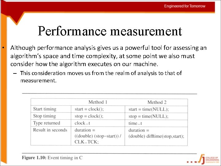
Performance measurement • Although performance analysis gives us a powerful tool for assessing an algorithm’s space and time complexity, at some point we also must consider how the algorithm executes on our machine. – This consideration moves us from the realm of analysis to that of measurement.

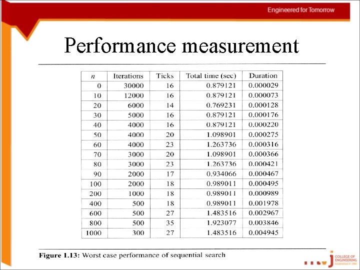
Performance measurement • Example 1. 22 [Worst case performance of the selection function]: – The tests were conducted on an IBM compatible PC with an 80386 cpu, an 80387 numeric coprocessor, and a turbo accelerator. We use Broland’s Turbo C compiler.

Performance measurement

Thank You. .